Deep learning is a hot topic these days. But what is it that makes it special and sets it apart from other aspects of machine learning? That is a deep question (pardon the pun). To even begin to answer it, we will need to learn the basics of neural networks.
Neural networks are the workhorses of deep learning. And while they may look like black boxes, deep down (sorry, I will stop the terrible puns) they are trying to accomplish the same thing as any other model — to make good predictions.
In this post, we will explore the ins and outs of a simple neural network. And by the end, hopefully you (and I) will have gained a deeper and more intuitive understanding of how neural networks do what they do.
The 30,000 Feet View
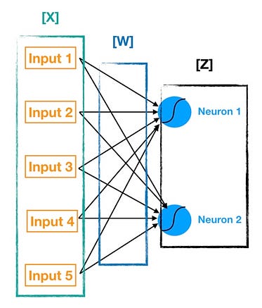
Let’s start with a really high level overview so we know what we are working with. Neural networks are multi-layer networks of neurons (the blue and magenta nodes in the chart below) that we use to classify things, make predictions, etc. Below is the diagram of a simple neural network with five inputs, 5 outputs, and two hidden layers of neurons.
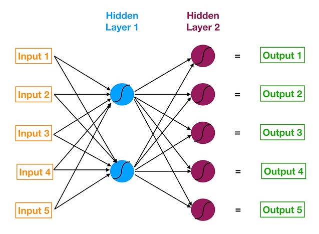
Neural network with two hidden layers
Starting from the left, we have:
- The input layer of our model in orange.
- Our first hidden layer of neurons in blue.
- Our second hidden layer of neurons in magenta.
- The output layer (a.k.a. the prediction) of our model in green.
The arrows that connect the dots shows how all the neurons are interconnected and how data travels from the input layer all the way through to the output layer.
Later we will calculate step by step each output value. We will also watch how the neural network learns from its mistake using a process known as backpropagation.
Getting our Bearings
But first let’s get our bearings. What exactly is a neural network trying to do? Like any other model, it’s trying to make a good prediction. We have a set of inputs and a set of target values — and we are trying to get predictions that match those target values as closely as possible.
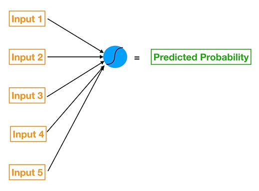
Forget for a second the more complicated looking picture of the neural network I drew above and focus on this simpler one below.
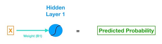
Logistic regression (with only one feature) implemented via a neural network
This is a single feature logistic regression (we are giving the model only one X variable) expressed through a neural network (if you need a refresher on logistic regression, I wrote about that here). To see how they connect we can rewrite the logistic regression equation using our neural network color codes.

Logistic regression equation
Let’s examine each element:
- X (in orange) is our input, the lone feature that we give to our model in order to calculate a prediction.
- B1 (in turquoise, a.k.a. blue-green) is the estimated slope parameter of our logistic regression — B1 tells us by how much the Log_Odds change as X changes. Notice that B1 lives on the turquoise line, which connects the input X to the blue neuron in Hidden Layer 1.
- B0 (in blue) is the bias — very similar to the intercept term from regression. The key difference is that in neural networks, every neuron has its own bias term (while in regression, the model has a singular intercept term).
- The blue neuron also includes a sigmoid activation function (denoted by the curved line inside the blue circle). Remember the sigmoid function is what we use to go from log-odds to probability (do a control-f search for “sigmoid” in my previous post).
- And finally we get our predicted probability by applying the sigmoid function to the quantity (B1*X + B0).
Not too bad right? So let’s recap. A super simple neural network consists of just the following components:
- A connection (though in practice, there will generally be multiple connections, each with its own weight, going into a particular neuron), with a weight “living inside it”, that transforms your input (using B1) and gives it to the neuron.
- A neuron that includes a bias term (B0) and an activation function (sigmoid in our case).
And these two objects are the fundamental building blocks of the neural network. More complex neural networks are just models with more hidden layers and that means more neurons and more connections between neurons. And this more complex web of connections (and weights and biases) is what allows the neural network to “learn” the complicated relationships hidden in our data.
Let’s Add a Bit of Complexity Now
Now that we have our basic framework, let’s go back to our slightly more complicated neural network and see how it goes from input to output. Here it is again for reference:
Our slightly more complicated neural network
The first hidden layer consists of two neurons. So to connect all five inputs to the neurons in Hidden Layer 1, we need ten connections. The next image (below) shows just the connections between Input 1 and Hidden Layer 1.
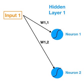
The connections between Input 1 and Hidden Layer 1
Note our notation for the weights that live in the connections — W1,1 denotes the weight that lives in the connection between Input 1 and Neuron 1 and W1,2 denotes the weight in the connection between Input 1 and Neuron 2. So the general notation that I will follow is Wa,b denotes the weight on the connection between Input a (or Neuron a) and Neuron b.
Now let’s calculate the outputs of each neuron in Hidden Layer 1 (known as the activations). We do so using the following formulas (W denotes weight, In denotes input).
Z1 = W1*In1 + W2*In2 + W3*In3 + W4*In4 + W5*In5 + Bias_Neuron1
Neuron 1 Activation = Sigmoid(Z1)
We can use matrix math to summarize this calculation (remember our notation rules — for example, W4,2 denotes the weight that lives in the connection between Input 4 and Neuron 2):
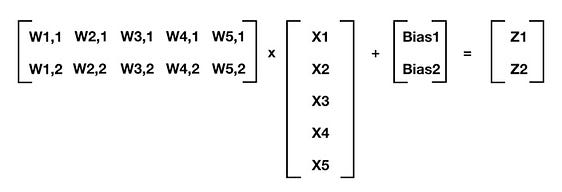
Matrix math makes our life easier
For any layer of a neural network where the prior layer is m elements deep and the current layer is n elements deep, this generalizes to:
[W] @ [X] + [Bias] = [Z]
Where [W] is your n by m matrix of weights (the connections between the prior layer and the current layer), [X] is your m by 1 matrix of either starting inputs or activations from the prior layer, [Bias] is your n by 1 matrix of neuron biases, and [Z] is your n by 1 matrix of intermediate outputs. In the previous equation, I follow Python notation and use @ to denote matrix multiplication. Once we have [Z], we can apply the activation function (sigmoid in our case) to each element of [Z] and that gives us our neuron outputs (activations) for the current layer.
Finally before we move on, let’s visually map each of these elements back onto our neural network chart to tie it all up ([Bias] is embedded in the blue neurons).
Visualizing [W], [X], and [Z]
By repeatedly calculating [Z] and applying the activation function to it for each successive layer, we can move from input to output. This process is known as forward propagation. Now that we know how the outputs are calculated, it’s time to start evaluating the quality of the outputs and training our neural network.
Time for the Neural Network to Learn
This is going to be a long post so feel free to take a coffee break now. Still with me? Awesome! Now that we know how a neural network’s output values are calculated, it is time to train it.
The training process of a neural network, at a high level, is like that of many other data science models — define a cost function and use gradient descent optimization to minimize it.
First let’s think about what levers we can pull to minimize the cost function. In traditional linear or logistic regression we are searching for beta coefficients (B0, B1, B2, etc.) that minimize the cost function. For a neural network, we are doing the same thing but at a much larger and more complicated scale.
In traditional regression, we can change any particular beta in isolation without impacting the other beta coefficients. So by applying small isolated shocks to each beta coefficient and measuring its impact on the cost function, it is relatively straightforward to figure out in which direction we need to move to reduce and eventually minimize the cost function.
Five feature logistic regression implemented via a neural network
In a neural network, changing the weight of any one connection (or the bias of a neuron) has a reverberating effect across all the other neurons and their activations in the subsequent layers.
That’s because each neuron in a neural network is like its own little model. For example, if we wanted a five feature logistic regression, we could express it through a neural network, like the one on the left, using just a singular neuron!
So each hidden layer of a neural network is basically a stack of models (each individual neuron in the layer acts like its own model) whose outputs feed into even more models further downstream (each successive hidden layer of the neural network holds yet more neurons).
The Cost Function
So given all this complexity, what can we do? It’s actually not that bad. Let’s take it step by step. First, let me clearly state our objective. Given a set of training inputs (our features) and outcomes (the target we are trying to predict):
We want to find the set of weights (remember that each connecting line between any two elements in a neural network houses a weight) and biases (each neuron houses a bias) that minimize our cost function — where the cost function is an approximation of how wrong our predictions are relative to the target outcome.
For training our neural network, we will use Mean Squared Error (MSE) as the cost function:
MSE = Sum [ ( Prediction - Actual )² ] * (1 / num_observations)
The MSE of a model tell us on average how wrong we are but with a twist — by squaring the errors of our predictions before averaging them, we punish predictions that are way off much more severely than ones that are just slightly off. The cost functions of linear regression and logistic regression operate in a very similar manner.
OK cool, we have a cost function to minimize. Time to fire up gradient descent right?
Not so fast — to use gradient descent, we need to know the gradient of our cost function, the vector that points in the direction of greatest steepness (we want to repeatedly take steps in the opposite direction of the gradient to eventually arrive at the minimum).
Except in a neural network we have so many changeable weights and biases that are all interconnected. How will we calculate the gradient of all of that? In the next section, we will see how backpropagation helps us deal with this problem.
Quick Review of Gradient Descent
The gradient of a function is the vector whose elements are its partial derivatives with respect to each parameter. For example, if we were trying to minimize a cost function, C(B0, B1), with just two changeable parameters, B0 and B1, the gradient would be:
Gradient of C(B0, B1) = [ [dC/dB0], [dC/dB1] ]
So each element of the gradient tells us how the cost function would change if we applied a small change to that particular parameter — so we know what to tweak and by how much. To summarize, we can march towards the minimum by following these steps:
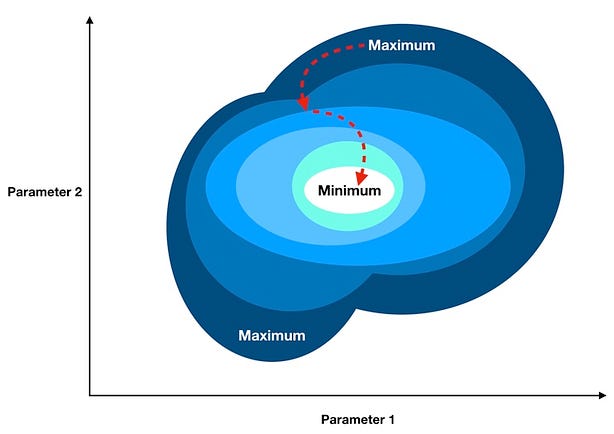
Illustration of Gradient Descent
- Compute the gradient of our “current location” (calculate the gradient using our current parameter values).
- Modify each parameter by an amount proportional to its gradient element and in the opposite direction of its gradient element. For example, if the partial derivative of our cost function with respect to B0 is positive but tiny and the partial derivative with respect to B1 is negative and large, then we want to decrease B0 by a tiny amount and increase B1 by a large amount to lower our cost function.
- Recompute the gradient using our new tweaked parameter values and repeat the previous steps until we arrive at the minimum.
Backpropagation
I will defer to this great textbook (online and free!) for the detailed math (if you want to understand neural networks more deeply, definitely check it out). Instead we will do our best to build an intuitive understanding of how and why backpropagation works.
Remember that forward propagation is the process of moving forward through the neural network (from inputs to the ultimate output or prediction). Backpropagation is the reverse. Except instead of signal, we are moving error backwards through our model.
Some simple visualizations helped a lot when I was trying to understand the backpropagation process. Below is my mental picture of a simple neural network as it forward propagates from input to output. The process can be summarized by the following steps:
- Inputs are fed into the blue layer of neurons and modified by the weights, bias, and sigmoid in each neuron to get the activations. For example: Activation_1 = Sigmoid( Bias_1 + W1*Input_1 )
- Activation 1 and Activation 2, which come out of the blue layer are fed into the magenta neuron, which uses them to produce the final output activation.
And the objective of forward propagation is to calculate the activations at each neuron for each successive hidden layer until we arrive at the output.
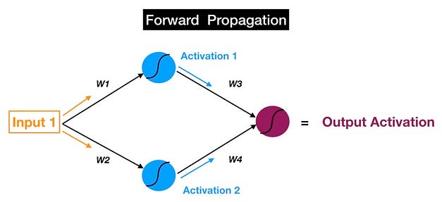
Forward propagation in a neural network
Now let’s just reverse it. If you follow the red arrows (in the picture below), you will notice that we are now starting at the output of the magenta neuron. That is our output activation, which we use to make our prediction, and the ultimate source of error in our model. We then move this error backwards through our model via the same weights and connections that we use for forward propagating our signal (so instead of Activation 1, now we have Error1 — the error attributable to the top blue neuron).
Remember we said that the goal of forward propagation is to calculate neuron activations layer by layer until we get to the output? We can now state the objective of backpropagation in a similar manner:
We want to calculate the error attributable to each neuron (I will just refer to this error quantity as the neuron’s error because saying “attributable” again and again is no fun) starting from the layer closest to the output all the way back to the starting layer of our model.
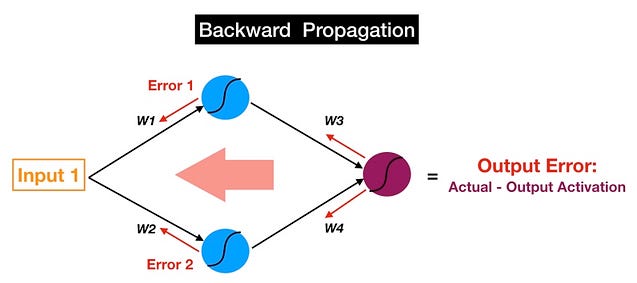
Backpropagation in a neural network
So why do we care about the error for each neuron? Remember that the two building blocks of a neural network are the connections that pass signals into a particular neuron (with a weight living in each connection) and the neuron itself (with a bias). These weights and biases across the entire network are also the dials that we tweak to change the predictions made by the model.
This part is really important:
The magnitude of the error of a specific neuron (relative to the errors of all the other neurons) is directly proportional to the impact of that neuron’s output (a.k.a. activation) on our cost function.
So the error of each neuron is a proxy for the partial derivative of the cost function with respect to that neuron’s inputs. This makes intuitive sense — if a particular neuron has a much larger error than all the other ones, then tweaking the weights and bias of our offending neuron will have a greater impact on our model’s total error than fiddling with any of the other neurons.
And the partial derivatives with respect to each weight and bias are the individual elements that compose the gradient vector of our cost function. So basically backpropagation allows us to calculate the error attributable to each neuron and that in turn allows us to calculate the partial derivatives and ultimately the gradient so that we can utilize gradient descent. Hurray!
An Analogy that Helps — The Blame Game
That’s a lot to digest so hopefully this analogy will help. Almost everyone has had a terrible colleague at some point in his or her life — someone who would always play the blame game and throw coworkers or subordinates under the bus when things went wrong.
Well neurons, via backpropagation, are masters of the blame game. When the error gets backpropagated to a particular neuron, that neuron will quickly and efficiently point the finger at the upstream colleague (or colleagues) who is most at fault for causing the error (i.e. layer 4 neurons would point the finger at layer 3 neurons, layer 3 neurons at layer 2 neurons, and so forth).
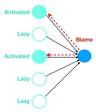
Neurons blame the most active upstream neurons
And how does each neuron know who to blame, as the neurons cannot directly observe the errors of other neurons? They just look at who sent them the most signal in terms of the highest and most frequent activations. Just like in real life, the lazy ones that play it safe (low and infrequent activations) skate by blame free while the neurons that do the most work get blamed and have their weights and biases modified. Cynical yes but also very effective for getting us to the optimal set of weights and biases that minimize our cost function. To the left is a visual of how the neurons throw each other under the bus.
And that in a nutshell is the intuition behind the backpropagation process. In my opinion, these are the three key takeaways for backpropagation:
- It is the process of shifting the error backwards layer by layer and attributing the correct amount of error to each neuron in the neural network.
- The error attributable to a particular neuron is a good approximation for how changing that neuron’s weights (from the connections leading into the neuron) and bias will affect the cost function.
- When looking backwards, the more active neurons (the non-lazy ones) are the ones that get blamed and tweaked by the backpropagation process.
Tying it All Together
If you have read all the way here, then you have my gratitude and admiration (for your persistence).
We started with a question, “What makes deep learning special?” I will attempt to answer that now (mainly from the perspective of basic neural networks and not their more advanced cousins like CNNs, RNNs, etc.). In my humble opinion, the following aspects make neural networks special:
- Each neuron is its own miniature model with its own bias and set of incoming features and weights.
- Each individual model/neuron feeds into numerous other individual neurons across all the hidden layers of the model. So we end up with models plugged into other models in a way where the sum is greater than its parts. This allows neural networks to fit all the nooks and crannies of our data including the nonlinear parts (but beware overfitting — and definitely consider regularization to protect your model from underperforming when confronted with new and out of sample data).
- The versatility of the many interconnected models approach and the ability of the backpropagation process to efficiently and optimally set the weights and biases of each model lets the neural network to robustly “learn” from data in ways that many other algorithms cannot.
Author’s Note: Neural networks and deep learning are extremely complicated subjects. I am still early in the process of learning about them. This blog was written as much to develop my own understanding as it was to help you, the reader. I look forward to all of your comments, suggestions, and feedback. Cheers!
More by me on Data Science Topics:
Sources: