In this article, we’ll take a look at the recent project I completed where I predicted the prices of used cars based on a number of factors. I found the dataset on Kaggle.
This project is special as I tried many different things and then finalized on the notebook that is included as part of the repository. I’ll explain each and every step I thought and how it turned out to be. The repository with the code is below:
Creating new features could be helpful e.g. I created the feature Manufacturer from Name.
Try different approaches to handle the same column. The Year column when used directly produced bad results so I instead used the age of each car derived from it which was much more useful. ``New_Price`` was first filled with average values based on ``Manufacturer`` but it was not useful, so I dropped the column in the second iteration.
Columns that seem irrelevant should be dropped. I dropped ``Index, Location, Name`` and ``New_Price`` .
Creating dummies requires handling of missing columns in test data.
Play around with the parameters of the ML model as it can be useful. The parameter ``n_estimators`` in RandomForestRegressor improved the ``r2_score`` when I set the value to 100. I also tried 1000 but it just took a lot longer without any noticeable improvement.
If you still want the complete details, keep reading!
Importar Librerias I’ll import ``datetime`` library to work with the ``Year`` column. The ``numpy`` and ``pandas`` libraries help me work with the dataset. ``matplotlib`` and ``seaborn`` help in plotting which I didn’t do much in this project. Finally, I import a number of things from ``sklearn`` especially metrics and models.
import datetime

import numpy as np
import pandas as pd

import matplotlib.pyplot as plt
import seaborn as sns
%matplotlib inline


from sklearn.model_selection import train_test_split
from sklearn.linear_model import LinearRegression
from sklearn.ensemble import RandomForestRegressor
from sklearn.preprocessing import StandardScaler
from sklearn.metrics import r2_score
Read dataset
The original Kaggle dataset had two files: ``train-data.csv`` and ``test-data.csv`` . However, the final output labels for the file ``test-data.csv`` were not given and hence, I would never be able to test my model. Thus, I decided to just work with the ``train-data.csv`` and rename it as ``dataset.csv`` inside the ``data`` folder.
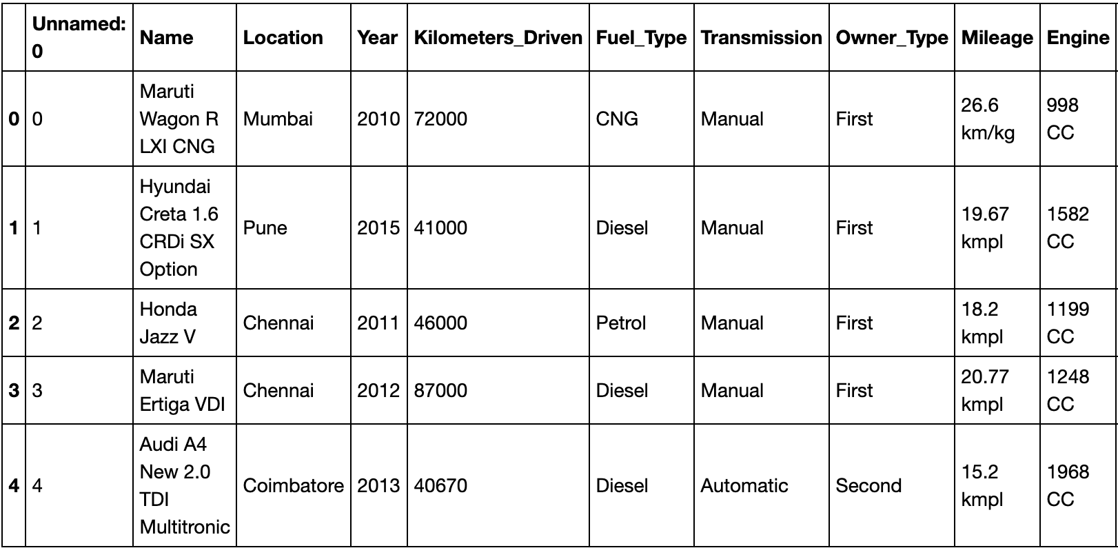
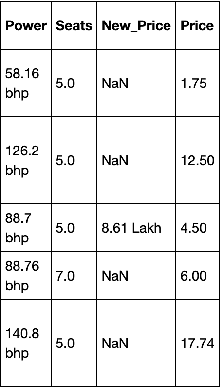
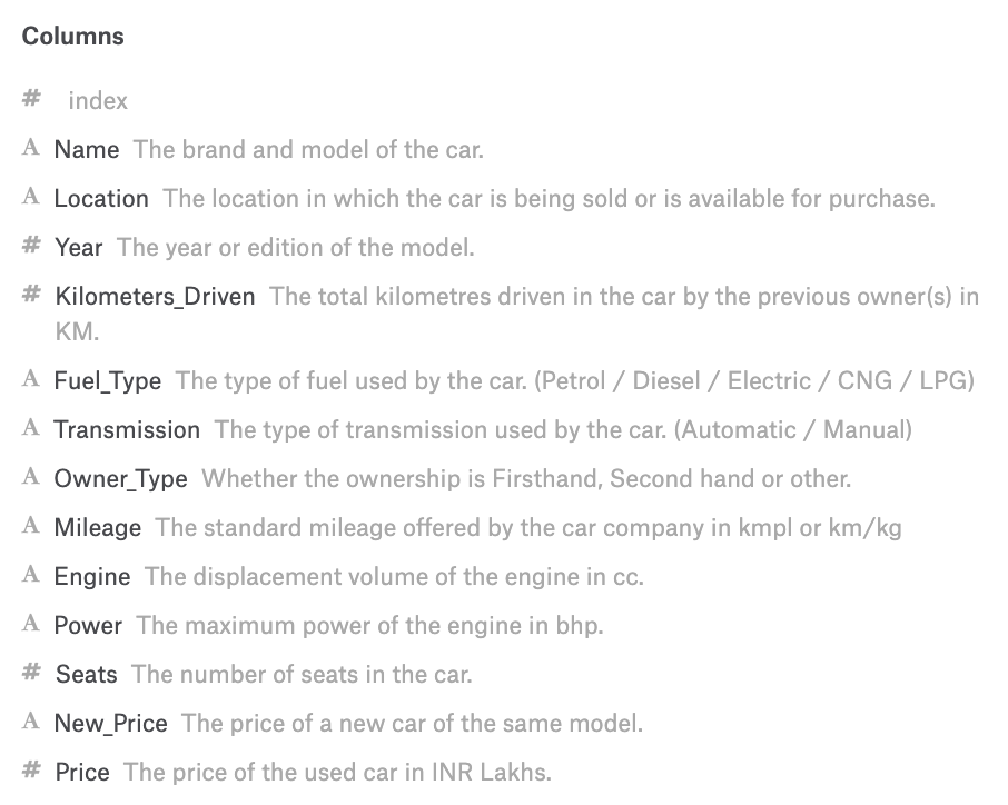
I output the training data information to see what the data looks like. We find that some columns like ``Mileage, Engine, Power`` and Seats have a few null values while ``New_Price`` has majority of its values missing. To get a better essence of what each column really represents, we can take a look at the Kaggle dashboard that has the data description.
Columns description
The dataset is now loaded and we know what each column means. It’s now time to do some exploratory analysis. Note that I will always work with training part and then transform the test part based on the training part only.
Exploratory Data Analysis Here, we’ll explore each of the columns above and discuss their relevance.
Index The first column in the dataset is unnamed. It is actually just an index for each row and thus, we can safely remove this column.
Name The ``Name`` column defines the name of each car. I thought the car name might not have a huge impact but the manufacturer of the car can. For example, if generally people find ``Maruti`` to produce reliable cars, their resale values should be higher. Thus, I decided to extract the ``Manufacturer`` from each ``Name`` . The first word of each ``Name`` is the manufacturer.
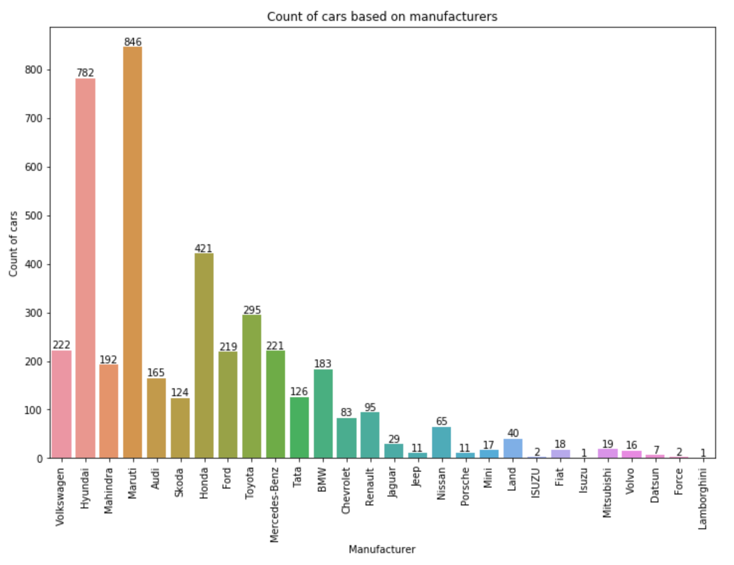
Let’s also plot and see the count of each cars based on the manufacturer.
plt.figure(figsize = (12, 8))
plot = sns.countplot(x = 'Manufacturer', data = X_train)
plt.xticks(rotation = 90)
for p in plot.patches:
     plot.annotate(p.get_height(),
                        (p.get_x() + p.get_width() / 2.0,
                         p.get_height()),
                        ha = 'center',
                        va = 'center',
                        xytext = (0, 5),
                        textcoords = 'offset points')


plt.title("Count of cars based on manufacturers")
plt.xlabel("Manufacturer")
plt.ylabel("Count of cars")
Manufacturer plot
As we can see in the plot above, Maruti has the maximum number of cars and Lamborghini has the least number of cars in the whole training data. Also, I don’t need the Name column so I dropped it.
Location I initially tried to use ``Location`` but it lead to many one hot columns without contributing much towards the prediction help. This means that location of selling has almost negligible effect on the final resale price of a car. Thus, I decided to drop this column.
Year I initially kept ``Year`` as it is to define the make of the model. But later did I realize that rather than the year, it’s how old the car is that has an effect on the resale value. Thus, taking cues from Kaggle, I decided to replace ``Year`` with the age of the car by subtracting the year from current year.
curr_time = datetime.datetime.now()
X_train['Year'] = X_train['Year'].apply(lambda x : curr_time.year - x)
X_test['Year'] = X_test['Year'].apply(lambda x : curr_time.year - x)
Fuel_Type, Transmission, and Owner_Type
All these columns are categorical columns. Thus, I’ll create dummy columns for each of these columns and use it for prediction.
The data output shows the high values that exist in the column. We should scale the data as well else columns like ``Kilometers_Driven`` can have a much stronger effect on prediction than other columns.
Mileage ``Mileage`` defines the mileage of the car. However, the mileage units vary based on the type of engine e.g. some are per Kg while some are per L. But for this case, we’ll consider them equivalent and just extract the numbers from this column.
Engine, Power y Seats The ``Engine`` values are defined in CC so I need to remove CC from the data. Similarly, ``Power`` has bhp, so I’ll remove bhp from it. Also, as there are missing values in all three, I’ll again replace them with the mean as I did for ``Mileage`` .
I use ``pd.to_numeric()`` as handles null values and does not produce errors when converting from string to numerical (int or float).
New_Price Most of the values in the column are missing. I initially decided to fill them up. I would fill the mean value based on the manufacturer. For example, for Ford, I’d take all values that are present, take their mean and then replace all null values of New_Price for Ford with that mean. However, this still left out a few null values. I would then fill these null values with mean of all the values in the column. The same was repeated for test data as well.
However, this approach wasn’t really successful. I tried to run the Random Forest Regressor on it and the results were very small ``r2_score`` values. Next, I decided that I would simply drop the column and the ``r2_score`` values improved significantly.
However, it is quite possible that due to lack of all types in test data, there may be missing columns. Let’s understand it with an example. For example in the column ``Transmission`` , the training data includes ``Manual`` and ``Automatic`` so the dummies would be like ``Transmission_Manual`` and ``Transmission_Automatic`` . But what if the test data has only ``Manual`` value and no ``Automatic`` one. In such a case, dummies would only lead to ``Transmission_Manual`` . This will leave the test dataset one column short in comparison to training data and the prediction won’t work. To handle this, we create columns in test data that are missing and fill them with zero. Finally, we order the test data just like train data.
missing_cols = set(X_train.columns) - set(X_test.columns)
for col in missing_cols:
    X_test[col] = 0
X_test = X_test[X_train.columns]
Training and predicting I’ll create a Linear Regression and a Random Forest model to train on the data and compare the ``r2_score`` values to select the best pick.
I get the ``r2_score`` for Linear Regression as 0.70 and for Random Forest as 0.88. Thus, Random Forest performed really well on the test data.
Conclusion In this article, we saw how to approach a machine learning problem in real life and how we might tweak features based on their relevance and the information they give out.
CreditsPredictive models have become a trusted advisor to many businesses and for a good reason. These models can “foresee the future”, and there are many different methods available, meaning any industry can find one that fits their particular challenges.When we talk about predictive models, we are talking either about a regression model (continuous output) or a classification model (nominal or binary output). In classification problems, we use two types of algorithms (dependent on the kind of output it creates):Class output: Algorithms like SVM and KNN create a class output. For instance, in a binary classification problem, the outputs will be either 0 or 1. However, today we have algorithms that can convert these class outputs to probability.Probability output: Algorithms like Logistic Regression, Random Forest, Gradient Boosting, Adaboost, etc. give probability outputs. Converting probability outputs to class output is just a matter of creating a threshold probability.IntroductionWhile data preparation and training a machine learning model is a key step in the machine learning pipeline, it’s equally important to measure the performance of this trained model. How well the model generalizes on the unseen data is what defines adaptive vs non-adaptive machine learning models.By using different metrics for performance evaluation, we should be in a position to improve the overall predictive power of our model before we roll it out for production on unseen data.Without doing a proper evaluation of the ML model using different metrics, and depending only on accuracy, it can lead to a problem when the respective model is deployed on unseen data and can result in poor predictions.This happens because, in cases like these, our models don’t learn but instead memorize;hence, they cannot generalize well on unseen data.Model Evaluation MetricsLet us now define the evaluation metrics for evaluating the performance of a machine learning model, which is an integral component of any data science project. It aims to estimate the generalization accuracy of a model on the future (unseen/out-of-sample) data.Confusion MatrixA confusion matrix is a matrix representation of the prediction results of any binary testing that is often used to describe the performance of the classification model (or “classifier”) on a set of test data for which the true values are known.The confusion matrix itself is relatively simple to understand, but the related terminology can be confusing.Confusion matrix with 2 class labels.Each prediction can be one of the four outcomes, based on how it matches up to the actual value:True Positive (TP): Predicted True and True in reality.True Negative (TN): Predicted False and False in reality.False Positive (FP): Predicted True and False in reality.False Negative (FN): Predicted False and True in reality.Now let us understand this concept using hypothesis testing.A Hypothesis is speculation or theory based on insufficient evidence that lends itself to further testing and experimentation. With further testing, a hypothesis can usually be proven true or false.A Null Hypothesis is a hypothesis that says there is no statistical significance between the two variables in the hypothesis. It is the hypothesis that the researcher is trying to disprove.We would always reject the null hypothesis when it is false, and we would accept the null hypothesis when it is indeed true.Even though hypothesis tests are meant to be reliable, there are two types of errors that can occur.These errors are known as Type 1 and Type II errors.For example, when examining the effectiveness of a drug, the null hypothesis would be that the drug does not affect a disease.Type I Error:- equivalent to False Positives(FP).The first kind of error that is possible involves the rejection of a null hypothesis that is true.Let’s go back to the example of a drug being used to treat a disease. If we reject the null hypothesis in this situation, then we claim that the drug does have some effect on a disease. But if the null hypothesis is true, then, in reality, the drug does not combat the disease at all. The drug is falsely claimed to have a positive effect on a disease.Type II Error:- equivalent to False Negatives(FN).The other kind of error that occurs when we accept a false null hypothesis. This sort of error is called a type II error and is also referred to as an error of the second kind.If we think back again to the scenario in which we are testing a drug, what would a type II error look like? A type II error would occur if we accepted that the drug hs no effect on disease, but in reality, it did.A sample python implementation of the Confusion matrix.import warnings import pandas as pd from sklearn import model_selection from sklearn.linear_model import LogisticRegression from sklearn.metrics import confusion_matrix import matplotlib.pyplot as plt %matplotlib inline #ignore warnings warnings.filterwarnings('ignore') # Load digits dataset url = "http://archive.ics.uci.edu/ml/machine-learning-databases/iris/iris.data" df = pd.read_csv(url) # df = df.values X = df.iloc[:,0:4] y = df.iloc[:,4] #test size test_size = 0.33 #generate the same set of random numbers seed = 7 #Split data into train and test set. X_train, X_test, y_train, y_test = model_selection.train_test_split(X, y, test_size=test_size, random_state=seed) #Train Model model = LogisticRegression() model.fit(X_train, y_train) pred = model.predict(X_test) #Construct the Confusion Matrix labels = ['Iris-setosa', 'Iris-versicolor', 'Iris-virginica'] cm = confusion_matrix(y_test, pred, labels) print(cm) fig = plt.figure() ax = fig.add_subplot(111) cax = ax.matshow(cm) plt.title('Confusion matrix') fig.colorbar(cax) ax.set_xticklabels([''] + labels) ax.set_yticklabels([''] + labels) plt.xlabel('Predicted Values') plt.ylabel('Actual Values') plt.show()Confusion matrix with 3 class labels.The diagonal elements represent the number of points for which the predicted label is equal to the true label, while anything off the diagonal was mislabeled by the classifier. Therefore, the higher the diagonal values of the confusion matrix the better, indicating many correct predictions.In our case, the classifier predicted all the 13 setosa and 18 virginica plants in the test data perfectly. However, it incorrectly classified 4 of the versicolor plants as virginica.There is also a list of rates that are often computed from a confusion matrix for a binary classifier:1. AccuracyOverall, how often is the classifier correct?Accuracy = (TP+TN)/totalWhen our classes are roughly equal in size, we can use accuracy, which will give us correctly classified values.Accuracy is a common evaluation metric for classification problems. It’s the number of correct predictions made as a ratio of all predictions made.Misclassification Rate(Error Rate): Overall, how often is it wrong. Since accuracy is the percent we correctly classified (success rate), it follows that our error rate (the percentage we got wrong) can be calculated as follows:Misclassification Rate = (FP+FN)/totalWe use the sklearn module to compute the accuracy of a classification task, as shown below.#import modules import warnings import pandas as pd import numpy as np from sklearn import model_selection from sklearn.linear_model import LogisticRegression from sklearn import datasets from sklearn.metrics import accuracy_score #ignore warnings warnings.filterwarnings('ignore') # Load digits dataset iris = datasets.load_iris() # # Create feature matrix X = iris.data # Create target vector y = iris.target #test size test_size = 0.33 #generate the same set of random numbers seed = 7 #cross-validation settings kfold = model_selection.KFold(n_splits=10, random_state=seed) #Model instance model = LogisticRegression() #Evaluate model performance scoring = 'accuracy' results = model_selection.cross_val_score(model, X, y, cv=kfold, scoring=scoring) print('Accuracy -val set: %.2f%% (%.2f)' % (results.mean()*100, results.std())) #split data X_train, X_test, y_train, y_test = model_selection.train_test_split(X, y, test_size=test_size, random_state=seed) #fit model model.fit(X_train, y_train) #accuracy on test set result = model.score(X_test, y_test) print("Accuracy - test set: %.2f%%" % (result*100.0))The classification accuracy is 88% on the validation set.2. PrecisionWhen it predicts yes, how often is it correct?Precision=TP/predicted yesWhen we have a class imbalance, accuracy can become an unreliable metric for measuring our performance. For instance, if we had a 99/1 split between two classes, A and B, where the rare event, B, is our positive class, we could build a model that was 99% accurate by just saying everything belonged to class A. Clearly, we shouldn’t bother building a model if it doesn’t do anything to identify class B; thus, we need different metrics that will discourage this behavior. For this, we use precision and recall instead of accuracy.3. Recall or SensitivityWhen it’s actually yes, how often does it predict yes?True Positive Rate = TP/actual yesRecall gives us the true positive rate (TPR), which is the ratio of true positives to everything positive.In the case of the 99/1 split between classes A and B, the model that classifies everything as A would have a recall of 0% for the positive class, B (precision would be undefined — 0/0). Precision and recall provide a better way of evaluating model performance in the face of a class imbalance. They will correctly tell us that the model has little value for our use case.Just like accuracy, both precision and recall are easy to compute and understand but require thresholds. Besides, precision and recall only consider half of the confusion matrix:4. F1 ScoreThe F1 score is the harmonic mean of the precision and recall, where an F1 score reaches its best value at 1 (perfect precision and recall) and worst at 0.Why harmonic mean? Since the harmonic mean of a list of numbers skews strongly toward the least elements of the list, it tends (compared to the arithmetic mean) to mitigate the impact of large outliers and aggravate the impact of small ones.An F1 score punishes extreme values more. Ideally, an F1 Score could be an effective evaluation metric in the following classification scenarios:When FP and FN are equally costly — meaning they miss on true positives or find false positives — both impact the model almost the same way, as in our cancer detection classification exampleAdding more data doesn’t effectively change the outcome effectivelyTN is high (like with flood predictions, cancer predictions, etc.)A sample python implementation of the F1 score.import warnings import pandas from sklearn import model_selection from sklearn.linear_model import LogisticRegression from sklearn.metrics import log_loss from sklearn.metrics import precision_recall_fscore_support as score, precision_score, recall_score, f1_score warnings.filterwarnings('ignore') url = "https://raw.githubusercontent.com/jbrownlee/Datasets/master/pima-indians-diabetes.data.csv" dataframe = pandas.read_csv(url) dat = dataframe.values X = dat[:,:-1] y = dat[:,-1] test_size = 0.33 seed = 7 model = LogisticRegression() #split data X_train, X_test, y_train, y_test = model_selection.train_test_split(X, y, test_size=test_size, random_state=seed) model.fit(X_train, y_train) precision = precision_score(y_test, pred) print('Precision: %f' % precision) # recall: tp / (tp + fn) recall = recall_score(y_test, pred) print('Recall: %f' % recall) # f1: tp / (tp + fp + fn) f1 = f1_score(y_test, pred) print('F1 score: %f' % f1)5. SpecificityWhen it’s no, how often does it predict no?True Negative Rate=TN/actual noIt is the true negative rate or the proportion of true negatives to everything that should have been classified as negative.Note that, together, specificity and sensitivity consider the full confusion matrix:6. Receiver Operating Characteristics (ROC) CurveMeasuring the area under the ROC curve is also a very useful method for evaluating a model. By plotting the true positive rate (sensitivity) versus the false-positive rate (1 — specificity), we get the Receiver Operating Characteristic (ROC) curve. This curve allows us to visualize the trade-off between the true positive rate and the false positive rate.The following are examples of good ROC curves. The dashed line would be random guessing (no predictive value) and is used as a baseline; anything below that is considered worse than guessing. We want to be toward the top-left corner:A sample python implementation of the ROC curves.#Classification Area under curve import warnings import pandas from sklearn import model_selection from sklearn.linear_model import LogisticRegression from sklearn.metrics import roc_auc_score, roc_curve warnings.filterwarnings('ignore') url = "https://raw.githubusercontent.com/jbrownlee/Datasets/master/pima-indians-diabetes.data.csv" dataframe = pandas.read_csv(url) dat = dataframe.values X = dat[:,:-1] y = dat[:,-1] seed = 7 #split data X_train, X_test, y_train, y_test = model_selection.train_test_split(X, y, test_size=test_size, random_state=seed) model.fit(X_train, y_train) # predict probabilities probs = model.predict_proba(X_test) # keep probabilities for the positive outcome only probs = probs[:, 1] auc = roc_auc_score(y_test, probs) print('AUC - Test Set: %.2f%%' % (auc*100)) # calculate roc curve fpr, tpr, thresholds = roc_curve(y_test, probs) # plot no skill plt.plot([0, 1], [0, 1], linestyle='--') # plot the roc curve for the model plt.plot(fpr, tpr, marker='.') plt.xlabel('False positive rate') plt.ylabel('Sensitivity/ Recall') # show the plot plt.show()In the example above, the AUC is relatively close to 1 and greater than 0.5. A perfect classifier will have the ROC curve go along the Y-axis and then along the X-axisLog LossLog Loss is the most important classification metric based on probabilities.As the predicted probability of the true class gets closer to zero, the loss increases exponentially:It measures the performance of a classification model where the prediction input is a probability value between 0 and 1. Log loss increases as the predicted probability diverge from the actual label. The goal of any machine learning model is to minimize this value. As such, smaller log loss is better, with a perfect model having a log loss of 0.A sample python implementation of the Log Loss.#Classification LogLoss import warnings import pandas from sklearn import model_selection from sklearn.linear_model import LogisticRegression from sklearn.metrics import log_loss warnings.filterwarnings('ignore') url = "https://raw.githubusercontent.com/jbrownlee/Datasets/master/pima-indians-diabetes.data.csv" dataframe = pandas.read_csv(url) dat = dataframe.values X = dat[:,:-1] y = dat[:,-1] seed = 7 #split data X_train, X_test, y_train, y_test = model_selection.train_test_split(X, y, test_size=test_size, random_state=seed) model.fit(X_train, y_train) #predict and compute logloss pred = model.predict(X_test) accuracy = log_loss(y_test, pred) print("Logloss: %.2f" % (accuracy))Logloss: 8.02
Jaccard IndexJaccard Index is one of the simplest ways to calculate and find out the accuracy of a classification ML model. Let’s understand it with an example. Suppose we have a labeled test set, with labels as –y = [0,0,0,0,0,1,1,1,1,1]And our model has predicted the labels as –y1 = [1,1,0,0,0,1,1,1,1,1]The above Venn diagram shows us the labels of the test set and the labels of the predictions, and their intersection and union.Jaccard Index or Jaccard similarity coefficient is a statistic used in understanding the similarities between sample sets. The measurement emphasizes the similarity between finite sample sets and is formally defined as the size of the intersection divided by the size of the union of the two labeled sets, with formula as –Jaccard Index or Intersection over Union(IoU)So, for our example, we can see that the intersection of the two sets is equal to 8 (since eight values are predicted correctly) and the union is 10 + 10–8 = 12. So, the Jaccard index gives us the accuracy as –So, the accuracy of our model, according to Jaccard Index, becomes 0.66, or 66%.Higher the Jaccard index higher the accuracy of the classifier.A sample python implementation of the Jaccard index.import numpy as np def compute_jaccard_similarity_score(x, y): intersection_cardinality = len(set(x).intersection(set(y))) union_cardinality = len(set(x).union(set(y))) return intersection_cardinality / float(union_cardinality) score = compute_jaccard_similarity_score(np.array([0, 1, 2, 5, 6]), np.array([0, 2, 3, 5, 7, 9])) print "Jaccard Similarity Score : %s" %score passJaccard Similarity Score : 0.375Kolomogorov Smirnov chartK-S or Kolmogorov-Smirnov chart measures the performance of classification models. More accurately, K-S is a measure of the degree of separation between positive and negative distributions.The cumulative frequency for the observed and hypothesized distributions is plotted against the ordered frequencies. The vertical double arrow indicates the maximal vertical difference.The K-S is 100 if the scores partition the population into two separate groups in which one group contains all the positives and the other all the negatives. On the other hand, If the model cannot differentiate between positives and negatives, then it is as if the model selects cases randomly from the population. The K-S would be 0.In most classification models the K-S will fall between 0 and 100, and that the higher the value the better the model is at separating the positive from negative cases.The K-S may also be used to test whether two underlying one-dimensional probability distributions differ. It is a very efficient way to determine if two samples are significantly different from each other.A sample python implementation of the Kolmogorov-Smirnov.from scipy.stats import kstest import random # N = int(input("Enter number of random numbers: ")) N = 10 actual =[] print("Enter outcomes: ") for i in range(N): # x = float(input("Outcomes of class "+str(i + 1)+": ")) actual.append(random.random()) print(actual) x = kstest(actual, "norm") print(x)The Null hypothesis used here assumes that the numbers follow the normal distribution. It returns statistics and p-value. If the p-value is < alpha, we reject the Null hypothesis.Alpha is defined as the probability of rejecting the null hypothesis given the null hypothesis(H0) is true. For most of the practical applications, alpha is chosen as 0.05.Gain and Lift ChartGain or Lift is a measure of the effectiveness of a classification model calculated as the ratio between the results obtained with and without the model. Gain and lift charts are visual aids for evaluating the performance of classification models. However, in contrast to the confusion matrix that evaluates models on the whole population gain or lift chart evaluates model performance in a portion of the population.The higher the lift (i.e. the further up it is from the baseline), the better the model.The following gains chart, run on a validation set, shows that with 50% of the data, the model contains 90% of targets, Adding more data adds a negligible increase in the percentage of targets included in the model.Gain/lift chartLift charts are often shown as a cumulative lift chart, which is also known as a gains chart. Therefore, gains charts are sometimes (perhaps confusingly) called “lift charts”, but they are more accurately cumulative lift charts.It is one of their most common uses is in marketing, to decide if a prospective client is worth calling.Gini CoefficientThe Gini coefficient or Gini Index is a popular metric for imbalanced class values. The coefficient ranges from 0 to 1 where 0 represents perfect equality and 1 represents perfect inequality. Here, if the value of an index is higher, then the data will be more dispersed.Gini coefficient can be computed from the area under the ROC curve using the following formula:Gini Coefficient = (2 * ROC_curve) — 1ConclusionUnderstanding how well a machine learning model is going to perform on unseen data is the ultimate purpose behind working with these evaluation metrics. Metrics like accuracy, precision, recall are good ways to evaluate classification models for balanced datasets, but if the data is imbalanced and there’s a class disparity, then other methods like ROC/AUC, Gini coefficient perform better in evaluating the model performance.Well, this concludes this article. I hope you guys have enjoyed reading it, feel free to share your comments/thoughts/feedback in the comment section.Thanks for reading !!!
DataSource AI announces the launch of the KTM AG inaugural AI Challenge, an unprecedented 3-month online competition that aims to revolutionise two-wheeler innovation through artificial intelligence and deep learning. KTM AG is a global frontrunner in two-wheeler innovation, known for pushing the boundaries of what's possible in the world of motorcycles. With a rich history of groundbreaking engineering and a commitment to cutting-edge technology, KTM AG has set new standards in performance, design, and safety. As a global leader in two-wheeler innovation, KTM AG invites participants to embark on this groundbreaking innovation journey. At the core of this competition lies a challenge set to redefine the future of motorcycle lighting systems. Participants are tasked with developing an algorithm for a high-beam lighting system utilizing a pixel matrix. Participants can find detailed guidelines in the Datathon competition. The datathon unfolds in a 3-tiered cascade model: This Code Challenge by KTM AG promises not only substantial rewards but also an exciting opportunity to shape the future of two-wheeler technology, along with supporting the participants to upscale and test their knowledge in a global AI competition. The cumulative budget for this remarkable Code Challenge by KTM AG is a substantial €24,000, motivating participants with not only the opportunity to push the boundaries of two-wheeler technology but also significant rewards for those who rise to the occasion. With cumulative prizes, contestants have the chance to potentially take home a maximum reward of €10,800 in addition to contributing to cutting-edge advancements in the field. We invite all aspiring innovators, data scientists, and AI enthusiasts to join us in this journey to "Code the Light Fantastic." For more information, rules, and registration details, please register hereAbout DataSource: At DataSource AI, we are driven by a singular mission - to democratise the immense power of data science and AI/ML for businesses of all sizes and budgets. We facilitate AI competitions, for businesses of all sizes and budgets by harnessing our extensive data expert community that's collaborating over our intelligent AI algorithm crowdsourcing platform. Our community is at the heart of what we do. We've built a diverse and talented pool of data experts who are passionate about solving real-world problems. They collaborate, ideate, and innovate, driving forward the frontiers of data science.
In our fast-paced digital world, we're producing staggering volumes of data every day. This data falls into two key categories: structured, known for its order and efficiency, and unstructured, a captivating puzzle brimming with untapped potential.In this article, we will uncover how AI confronts the complexities of unstructured data, the hurdles it faces, and the intriguing opportunities it opens up to businesses from any kind of industry.Understanding Unstructured DataUnstructured data mining is the technique of extracting valuable and meaningful insights from an abundant well of unstructured data. It uncovers hidden gems of knowledge, making it a crucial pursuit in our data-rich era.In today's digital realm, unstructured data is generated in unprecedented quantities. Billions of text documents, images, and videos come to life daily, creating a treasure trove of information just waiting for organizations to explore.Unlocking the insights hidden within unstructured data can provide organizations with a competitive edge. This data can reveal customer sentiments, emerging trends, and valuable feedback that might otherwise go unnoticed.The Basics of Data MiningHow data mining works is that it discovers patterns, trends, and valuable information within a dataset. It involves various techniques to extract knowledge from raw data. While it's exceptionally effective with structured data, applying data mining to unstructured data requires a unique set of skills and tools.Unstructured Data MiningUnstructured data mining is a method focused on the extraction of valuable information from the vast, unstructured data available. This process uncovers hidden insights, making it a valuable endeavor in today's data-driven world.The AI RevolutionThe AI revolution has given rise to an exciting era of possibilities in unstructured data mining. AI's remarkable capabilities are instrumental in taming the unstructured data landscape, and it involves a multitude of components, including:Machine learning enables AI systems to learn from data, make predictions, and identify patterns, enhancing data mining capabilities.Deep learning uses neural networks to model complex patterns in unstructured data, which is particularly valuable in image and speech recognition.Sentiment analysis gauges emotional tones within textual data, helping to understand public opinion and tailor strategies.Pattern recognition identifies recurring structures in data, aiding in image processing and text mining.Knowledge graphs structure data relationships, improving contextual understanding and data retrieval.Anomaly detection identifies outliers in data, which is essential for fraud detection and data security.Challenges in Unstructured Data MiningAs promising as AI is at handling unstructured data, it's not without its set of challenges. Here, we delve into some of the major hurdles:Data QualityUnstructured data is inherently messy. It's laden with errors, inconsistencies, and biases, which makes it a challenge to extract meaningful insights from this data. AI systems need to be trained rigorously to navigate and decipher this diversity in data quality. Techniques like data cleansing, normalization, and the use of context are essential in ensuring that AI systems provide accurate results.ScalabilityAs the volume of unstructured data grows, AI systems must scale to handle the data influx effectively. Traditional hardware and algorithms might not be sufficient to handle this data influx. Scalable infrastructure and distributed computing become crucial to ensuring that AI systems can process and analyze vast amounts of data efficiently.Privacy ConcernsMining unstructured data often raises ethical questions regarding privacy and data protection. That’s why it’s essential to strike the right balance between data utilization and respecting individual privacy. It's a challenge to ensure that AI systems are used responsibly and in compliance with data protection laws and regulations, such as GDPR in Europe. Techniques like anonymization and consent management play a vital role in addressing these privacy concerns.Opportunities and ApplicationsAI's role in unstructured data mining has opened up a world of opportunities across various industries. Let's explore some of the most promising applications:Customer InsightsUnstructured data, particularly sourced from social media and customer reviews, serves as a goldmine of information on customer behavior and preferences. By leveraging AI algorithms, companies can analyze sentiments, spot emerging trends, and even forecast future buying patterns. With these insights, they can fine-tune their marketing strategies, product development, and customer service to align with their ever-evolving audience's demands.Healthcare DiagnosisThe abundance of unstructured data found in medical records, radiological images, and wearable device data holds the key to transformative advancements. AI-powered systems, known for their proficiency in the analysis of this data, not only facilitate early disease detection but also provide highly individualized treatment plans, ultimately raising the standard of patient care. For example: AI expedites the process of analyzing medical images for anomalies, resulting in a significant reduction in the time required for diagnosing and treating severe conditions.Fraud DetectionWhen it comes to financial institutions, AI is a vital tool for exposing fraudulent activities that often hide within the vast volumes of unstructured transaction data. Through a meticulous examination of transaction patterns and anomalies, AI systems can rapidly pinpoint fraudulent actions, providing businesses with a robust defense against significant financial losses. The ability to detect and thwart fraud in real-time provides a critical advantage, resulting in annual savings of billions of dollars for businesses.ConclusionThe future belongs to those who embrace the AI revolution in unstructured data mining. In this future, data isn't just information; it's the key to success. So, let's move forward, embracing this tomorrow, where possibilities are limitless and opportunities are endless.
In the age of digital marketing and content creation, data-driven creativity is becoming an increasingly important concept. It's the fusion of artistic vision with the insights gleaned from data science to enhance the impact and effectiveness of video content. This 2500-word blog will explore how data science can be leveraged to elevate video content creation, ensuring that it not only engages but also resonates with the intended audience.Introduction to Data-Driven CreativityData-driven creativity marks a groundbreaking shift in video content creation, blending artistic vision with the insights provided by data science. This combination allows creators to break free from conventional creative limits, using data analytics to develop content that is both visually captivating and strategically significant. By delving into viewer behavior, preferences, and interactions, creators can refine their stories and visuals, achieving a deeper connection with their audience. This technique effectively transforms data into a guide for storytelling, steering content towards increased relevance and attractiveness. Consequently, video content becomes a more potent medium for engaging viewers and delivering impactful messages. Fundamentally, data-driven creativity is about converting data points into compelling stories and turning analytical insights into creative masterpieces, thereby redefining the standards of digital video content.Understanding the Role of Data in Video Content CreationExploring the Role of Data in Video Content Creation ventures into the rapidly growing realm of data-driven creativity, where data science emerges as a key instrument in enriching video content. In this realm, data transcends mere figures to become a narrative element, providing rich insights into what audiences prefer, how they behave, and emerging trends. Utilizing data, video creators can break free from conventional creative constraints, shaping their stories to more deeply connect with viewers. This process involves a detailed examination of viewer interactions, demographics, and feedback to hone storytelling skills, aiming to create videos that are not only watched but also emotionally impactful and memorable. Data-driven creativity is a fusion of art and science, where each view, reaction, and comment plays a role in directing the trajectory of video content, enhancing its relevance, engagement, and effect. This marks a transformative phase in content creation, where data equips creators to weave narratives that are not just creatively rich but also finely tuned to the dynamic preferences and interests of their audience.The Process of Gathering and Analyzing DataCollecting and analyzing data forms the foundation of data-driven creativity, especially in the realm of video content enhancement. This process involves the acquisition of key information, including audience demographics, interaction metrics, and performance measures, utilizing sophisticated tools and technologies. These range from social media analytics to advanced data mining applications designed to track a broad spectrum of viewer interactions. Once collected, this data undergoes thorough analysis to identify trends, preferences, and behaviors within the target audience. Such analysis equips content creators with insightful knowledge, allowing them to adjust their video content for greater appeal and connection with their audience. Leveraging these insights, creators can modify elements such as the tone, style, and themes of their content, revolutionizing storytelling methods and ensuring their content is both captivating and impactful. This integration of data science with creative storytelling heralds a transformative phase in video content production, where analytical findings significantly enhance artistic expression.Tailoring Content to Audience PreferencesAdapting content to audience preferences through data-driven creativity signifies a vital evolution in video content production. By incorporating data science, creators gain profound insights into audience behaviors, likes, and engagement patterns. This approach facilitates the creation of content that better resonates with viewers, ensuring everything from the plot to visual elements aligns with their interests. Utilizing analytics such as viewer habits and interaction rates, creators can pinpoint engaging aspects for better video content. Using a high-quality video editor tool is important to make the video look better. This knowledge allows precise adjustments, making the content not only captivating but also highly relevant. Ultimately, incorporating data in video content creation leads to more impactful and resonant viewer experiences, forging a deeper bond between the audience and the content.Enhancing Storytelling with Data InsightsUtilizing data insights to enhance storytelling is a groundbreaking method in video content production. Termed data-driven creativity, this technique blends the storytelling craft with data science accuracy. Content creators leverage analysis of viewer engagement, preferences, and behavior to fine-tune their narratives, ensuring a deeper connection with their audience. This integration results in not only engaging narratives but also ones that are in tune with audience interests and emerging trends. Insights from data grant a clearer understanding of what truly engages viewers, empowering creators to optimize their storytelling for the greatest effect. This modern approach reinvents traditional storytelling into an experience that's both more impactful and centered around the audience, with each creative decision being shaped and enriched by data.Using Data to Predict Future TrendsUtilizing data for future trends in data-driven creativity marks a revolutionary step in improving video content via data science. This technique focuses on analyzing viewer interactions, demographic information, and behavioral tendencies to predict future content direction. Using data enables creators to be proactive, crafting video content that resonates with emerging audience preferences and interests. Such a forward-thinking approach guarantees ongoing relevance in a dynamic digital world and fosters innovation and leadership among content creators. The blend of data analytics and artistic insight leads to the production of not just captivating but also pioneering videos, demonstrating the significant role of data in shaping the future of video content creation.Balancing Creativity and DataAchieving a harmonious blend of creativity and data in video content production is both subtle and potent. Data-driven creativity embodies the convergence of artistic flair and data analytics, providing an innovative method to boost video effectiveness. By weaving in data analysis, video creators unlock insights into what their audience prefers and how they behave, guiding their artistic choices. This integration results in content that is not only enthralling but also deeply meaningful to viewers. It is essential, however, to ensure that data serves as a guide, not a ruler, in the creative journey. This equilibrium keeps the content fresh and appealing while aligning it thoughtfully with data-driven knowledge. In essence, data-driven creativity in video content merges the narrative craft with analytical insights, culminating in videos that are both compelling and influential.Overcoming Challenges in Data-Driven CreativityOvercoming hurdles in data-driven creativity necessitates a nuanced integration of data science into the creation of video content. It involves striking a delicate balance between analytical methodologies and artistic expression, ensuring that data serves as an informative tool rather than a constraint on creativity. Accurate interpretation of data empowers content creators to avoid formulaic outputs, utilizing insights to enrich storytelling and enhance audience engagement. This intricate process demands a comprehensive understanding of the artistry of video creation and the scientific principles behind data analysis. Ethical considerations, including respecting audience privacy and obtaining data consent, are pivotal in this approach. Innovative strategies within data-driven creativity empower creators to produce content that forges deeper connections with viewers, setting new benchmarks in the digital landscape. Embracing these challenges is essential for unlocking the full potential of data-enhanced video content.Ethical Considerations in Data-Driven CreativityIn the domain of data-driven creativity, ethical considerations play a crucial role, especially when utilizing data science to enhance video content. While utilizing data insights can enhance creative processes, it is essential to address privacy concerns and ensure transparent, responsible data usage. Achieving the right equilibrium between creativity and ethical considerations becomes paramount as brands employ data to customize video content. Upholding user privacy and securing informed consent are fundamental principles in ethical data-driven creativity, fostering trust among audiences. Moreover, there is an obligation to avoid perpetuating biases and stereotypes in content creation, championing inclusivity and diversity. Ethical practices not only maintain brand integrity but also contribute to a positive and respectful digital environment for consumers.Tools and Resources for Data-Driven Video CreationExplore the potential of data-driven creativity using state-of-the-art tools and resources for crafting videos. In the current digital landscape, integrating data science and video content is transforming the landscape of creative processes. Immerse yourself in a domain where insights derived from data direct every facet of video production. These tools empower creators to customize content according to audience preferences, ensuring that each video is not only visually captivating but also strategically aligned. From scriptwriting informed by analytics to incorporating personalized visual elements, the utilization of data science takes video content to unprecedented levels. Delve into the crossroads of technology and creativity, where strategies driven by data redefine storytelling, captivating audiences in a personalized and meaningful manner.The Future of Data-Driven Creativity in Video ContentThe evolution of data-driven creativity in video content is set to transform our interaction with digital media. Through the incorporation of data science, creators gain valuable insights into viewer preferences, behavior, and trends. This collaboration enables a personalized and captivating viewing experience, heightening audience engagement. With the utilization of data-driven creativity, content producers can shape videos to suit the unique preferences of their target audience, resulting in more impactful storytelling and brand communication. As technology progresses, we anticipate a shift towards highly personalized content, driven by data insights, leading to innovative approaches in video production. This convergence of creativity and data science holds significant promise for the future development of video content within the digital landscape.ConclusionIn summary, the convergence of data-driven insights and creative components represents a transformative shift in the realm of video content creation. The fusion of Data Science and creativity provides content producers with the tools to precisely tailor videos to audience preferences, resulting in more impactful and engaging content. Leveraging the potential of data facilitates a deeper comprehension of viewer behavior, enabling targeted storytelling. Amidst the digital landscape, the symbiosis of data and creativity not only elevates video content but also fosters innovation and personalized experiences. Looking ahead, embracing Data-Driven Creativity becomes crucial for maintaining a leading edge in the continually evolving landscape of video content creation.
nikos_datasource
May 25, 2020
Join our private community in Discord
Keep up to date by participating in our global community of data scientists and AI enthusiasts. We discuss the latest developments in data science competitions, new techniques for solving complex challenges, AI and machine learning models, and much more!