
Missing data is an everyday problem that a data professional need to deal with. Though there are many articles, blogs, videos already available, I found it is difficult to find a concise consolidated information in a single place. That’s why I am putting my effort here, hoping it will be useful to any data practitioner or enthusiast.
What is missing data? Missing data are defined as values that are not available and that would be meaningful if they are observed. Missing data can be anything from missing sequence, incomplete feature, files missing, information incomplete, data entry error etc. Most datasets in the real world contain missing data. Before you can use data with missing data fields, you need to transform those fields so they can be used for analysis and modelling. Like many other aspects of data science, this too may actually be more art than science. Understanding the data and the domain from which it comes is very important.
Having missing values in your data is not necessarily a setback but it is an opportunity to perform right feature engineering to guide the model to interpret the missing information right way. There are machine learning algorithms and packages that can automatically detect and deal with missing data, but it’s still recommended to transform the missing data manually through analysis and coding strategy. First, we need to understand what are the types of missing data. Missingness is broadly categorized in 3 categories:
Missing Completely at Random (MCAR)
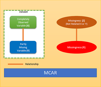
When we say data are missing completely at random, we mean that the missingness has nothing to do with the observation being studied (Completely Observed Variable (X) and Partly Missing Variable (Y)). For example, a weighing scale that ran out of batteries, a questionnaire might be lost in the post, or a blood sample might be damaged in the lab. MCAR is an ideal but unreasonable assumption. Generally, data are regarded as being MCAR when data are missing by design, because of an equipment failure or because the samples are lost in transit or technically unsatisfactory. The statistical advantage of data that are MCAR is that the analysis remains unbiased. A pictorial view of MCAR as below where missingness has no relation to dataset variables X or Y. Missingness is not related to X or Y but some other reason Z.
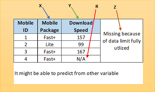
Let’s explore one example of mobile data. Here one sample has missing value which is not because of dataset variables but because of another reason.
Missing at Random (MAR)
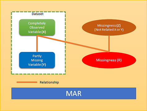
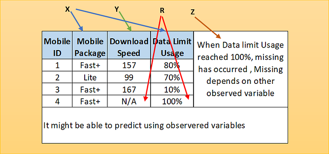
When we say data are missing at random, we mean that missing data on a partly missing variable (Y) is related to some other completely observed variables(X) in the analysis model but not to the values of Y itself.
It is not specifically related to the missing information. For example, if a child does not attend an examination because the child is ill, this might be predictable from other data we have about the child’s health, but it would not be related to what we would have examined had the child not been ill. Some may think that MAR does not present a problem. However, MAR does not mean that the missing data can be ignored. A pictorial view of MAR as below where missingness has relation to dataset variable X but not with Y. It can have other relation as well (Z).
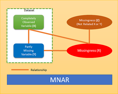
Missing not at Random (MNAR)
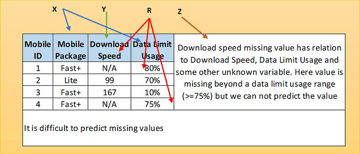
If the characters of the data do not meet those of MCAR or MAR, then they fall into the category of missing not at random (MNAR). When data are missing not at random, the missingness is specifically related to what is missing, e.g. a person does not attend a drug test because the person took drugs the night before, a person did not take English proficiency test due to his poor English language skill. The cases of MNAR data are problematic. The only way to obtain an unbiased estimate of the parameters in such a case is to model the missing data but that requires proper understanding and domain knowledge of the missing variable. The model may then be incorporated into a more complex one for estimating the missing values. A pictorial view of MNAR as below where missingness has direct relation to variable Y. It can have other relation as well (X & Z).
There are several strategies which can be applied to handle missing data to make the Machine Learning/Statistical Model.
Try to obtain the missing data
This may be possible in data collection phase in survey like situation where one can check if survey data is captured in entirety before respondent leaves the room. Sometimes it may be possible to reach out to the source to get the data like asking the missing question again for a response. In real world scenario, this is very unlikely way to resolve the missing data problem.
Educated Guessing
It sounds arbitrary and isn’t never preferred course of action, but one can sometimes infer a missing value based on other response. For related questions, for example, like those often presented in a matrix, if the participant responds with all “2s”, assume that the missing value is a 2.
Discard Data
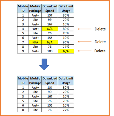
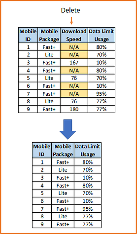
1) list-wise (Complete-case analysis — CCA) deletion
By far the most common approach to the missing data is to simply omit those cases with the missing data and analyse the remaining data. This approach is known as the complete case (or available case) analysis or list-wise deletion.
If there is a large enough sample, where power is not an issue, and the assumption of MCAR is satisfied, the listwise deletion may be a reasonable strategy. However, when there is not a large sample, or the assumption of MCAR is not satisfied, the listwise deletion is not the optimal strategy. It also introduces bias if it does not satisfy MCAR.
Refer to below sample observation after deletion
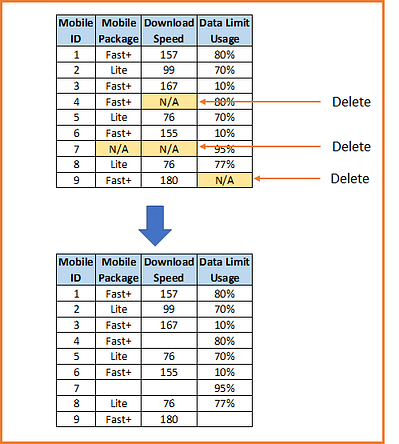
2) Pairwise (available case analysis — ACA) Deletion
In this case, only the missing observations are ignored and analysis is done on variables present. If there is missing data elsewhere in the data set, the existing values are used. Since a pairwise deletion uses all information observed, it preserves more information than the listwise deletion.
Pairwise deletion is known to be less biased for the MCAR or MAR data. However, if there are many missing observations, the analysis will be deficient. the problem with pairwise deletion is that even though it takes the available cases, one can’t compare analyses because the sample is different every time.
3) Dropping Variables
If there are too many data missing for a variable it may be an option to delete the variable or the column from the dataset. There is no rule of thumbs for this but depends on situation and a proper analysis of data is needed before the variable is dropped all together. This should be the last option and need to check if model performance improves after deletion of variable.
Retain All Data
The goal of any imputation technique is to produce a complete dataset that can then be then used for machine learning. There are few ways we can do imputation to retain all data for analysis and building the model.
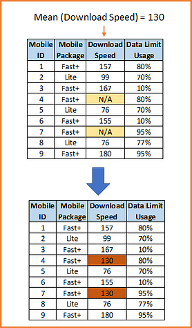
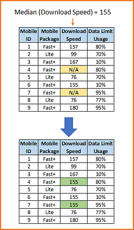
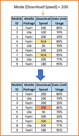
1) Mean, Median and Mode
In this imputation technique goal is to replace missing data with statistical estimates of the missing values. Mean, Median or Mode can be used as imputation value.
In a mean substitution, the mean value of a variable is used in place of the missing data value for that same variable. This has the benefit of not changing the sample mean for that variable. The theoretical background of the mean substitution is that the mean is a reasonable estimate for a randomly selected observation from a normal distribution. However, with missing values that are not strictly random, especially in the presence of a great inequality in the number of missing values for the different variables, the mean substitution method may lead to inconsistent bias. Distortion of original variance and Distortion of co-variance with remaining variables within the dataset are two major drawbacks of this method.
Median can be used when variable has a skewed distribution.
The rationale for Mode is to replace the population of missing values with the most frequent value, since this is the most likely occurrence.
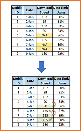
2) Last Observation Carried Forward (LOCF)
If data is time-series data, one of the most widely used imputation methods is the last observation carried forward (LOCF). Whenever a value is missing, it is replaced with the last observed value. This method is advantageous as it is easy to understand and communicate. Although simple, this method strongly assumes that the value of the outcome remains unchanged by the missing data, which seems unlikely in many settings.
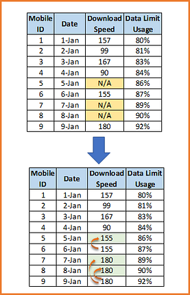
3) Next Observation Carried Backward (NOCB)
A similar approach like LOCF which works in the opposite direction by taking the first observation after the missing value and carrying it backward (“next observation carried backward”, or NOCB).
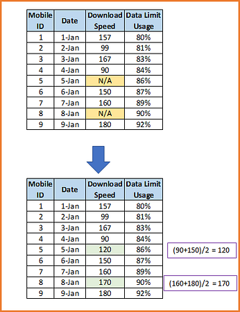
4) Linear Interpolation
Interpolation is a mathematical method that adjusts a function to data and uses this function to extrapolate the missing data. The simplest type of interpolation is the linear interpolation, that makes a mean between the values before the missing data and the value after. Of course, we could have a pretty complex pattern in data and linear interpolation could not be enough. There are several different types of interpolation. Just in Pandas we have the following options like : ‘linear’, ‘time’, ‘index’, ‘values’, ‘nearest’, ‘zero’, ‘slinear’, ‘quadratic’, ‘cubic’, ‘polynomial’, ‘spline’, ‘piece wise polynomial’ and many more .
5) Common-Point Imputation
For a rating scale, using the middle point or most commonly chosen value. For example, on a five-point scale, substitute a 3, the midpoint, or a 4, the most common value (in many cases). It is similar to mean value but more suitable for ordinal values.
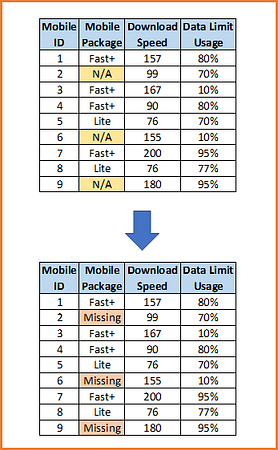
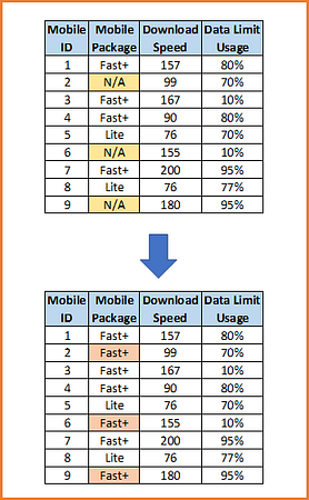
6) Adding a category to capture NA
This is perhaps the most widely used method of missing data imputation for categorical variables. This method consists in treating missing data as if they were an additional label or category of the variable. All the missing observations are grouped in the newly created label ‘Missing’. It does not assume anything on the missingness of the values. It is very well suited when the number of missing data is high.
7) Frequent category imputation
Replacement of missing values by the most frequent category is the equivalent of mean/median imputation. It consists of replacing all occurrences of missing values within a variable by the most frequent label or category of the variable.
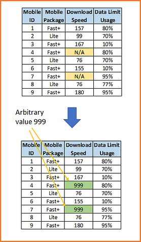
8) Arbitrary Value Imputation
Arbitrary value imputation consists of replacing all occurrences of missing values within a variable by an arbitrary value. Ideally arbitrary value should be different from the median/mean/mode, and not within the normal values of the variable. Typically used arbitrary values are 0, 999, -999 (or other combinations of 9’s) or -1 (if the distribution is positive). Sometime data already contain arbitrary value from originator for the missing values. This works reasonably well for numerical features that are predominantly positive in value, and for tree-based models in general. This used to be a more common method in the past when the out-of-the box machine learning libraries and algorithms were not very adept at working with missing data.
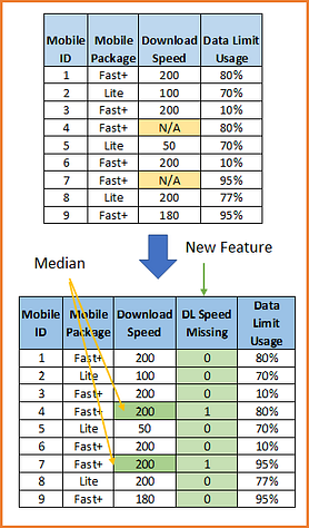
9) Adding a variable to capture NA
When data are not missing completely at random, we can capture the importance of missingness by creating an additional variable indicating whether the data was missing for that observation (1) or not (0). The additional variable is a binary variable: it takes only the values 0 and 1, 0 indicating that a value was present for that observation, and 1 indicating that the value was missing for that observation. Typically, mean/median imputation is done together with adding a variable to capture those observations where the data was missing.
10) Random Sampling Imputation
Random sampling imputation is in principle similar to mean/median imputation, in the sense that it aims to preserve the statistical parameters of the original variable, for which data is missing. Random sampling consists of taking a random observation from the pool of available observations of the variable, and using that randomly extracted value to fill the NA. In Random Sampling one takes as many random observations as missing values are present in the variable. Random sample imputation assumes that the data are missing completely at random (MCAR). If this is the case, it makes sense to substitute the missing values, by values extracted from the original variable distribution.
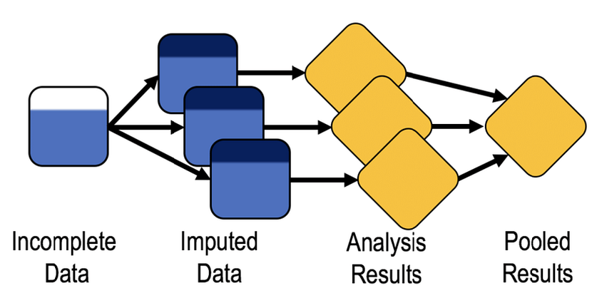
Multiple Imputation
Multiple Imputation (MI) is a statistical technique for handling missing data. The key concept of MI is to use the distribution of the observed data to estimate a set of plausible values for the missing data. Random components are incorporated into these estimated values to show their uncertainty. Multiple datasets are created and then analysed individually but identically to obtain a set of parameter estimates. Estimates are combined to obtain a set of parameter estimates. As a flexible way of handling more than one missing variable, apply a Multiple Imputation by Chained Equations (MICE) approach. The benefit of the multiple imputation is that in addition to restoring the natural variability of the missing values, it incorporates the uncertainty due to the missing data, which results in a valid statistical inference. Refer to reference section to get more information on MI and MICE. Below is a schematic representation of MICE.
Predictive/Statistical models that impute the missing data
This should be done in conjunction with some kind of cross-validation scheme in order to avoid leakage. This can be very effective and can help with the final model. There are many options for such predictive model including neural network. Here I am listing a few which are very popular.
Linear Regression
In regression imputation, the existing variables are used to make a prediction, and then the predicted value is substituted as if an actual obtained value. This approach has a number of advantages, because the imputation retains a great deal of data over the list wise or pair wise deletion and avoids significantly altering the standard deviation or the shape of the distribution. However, as in a mean substitution, while a regression imputation substitutes a value that is predicted from other variables, no novel information is added, while the sample size has been increased and the standard error is reduced.
Random Forest
Random forest is a non-parametric imputation method applicable to various variable types that works well with both data missing at random and not missing at random. Random forest uses multiple decision trees to estimate missing values and outputs OOB (out of bag) imputation error estimates. One caveat is that random forest works best with large datasets and using random forest on small datasets runs the risk of overfitting.
k-NN (k Nearest Neighbour)
k-NN imputes the missing attribute values on the basis of nearest K neighbour. Neighbours are determined on the basis of distance measure. Once K neighbours are determined, missing value are imputed by taking mean/median or mode of known attribute values of missing attribute.
Maximum likelihood
There are a number of strategies using the maximum likelihood method to handle the missing data. In these, the assumption that the observed data are a sample drawn from a multivariate normal distribution is relatively easy to understand. After the parameters are estimated using the available data, the missing data are estimated based on the parameters which have just been estimated.
Expectation-Maximization
Expectation-Maximization (EM) is a type of the maximum likelihood method that can be used to create a new data set, in which all missing values are imputed with values estimated by the maximum likelihood methods. This approach begins with the expectation step, during which the parameters (e.g., variances, co-variances, and means) are estimated, perhaps using the list wise deletion. Those estimates are then used to create a regression equation to predict the missing data. The maximization step uses those equations to fill in the missing data. The expectation step is then repeated with the new parameters, where the new regression equations are determined to “fill in” the missing data. The expectation and maximization steps are repeated until the system stabilizes.
Sensitivity analysis
Sensitivity analysis is defined as the study which defines how the uncertainty in the output of a model can be allocated to the different sources of uncertainty in its inputs. When analysing the missing data, additional assumptions on the reasons for the missing data are made, and these assumptions are often applicable to the primary analysis. However, the assumptions cannot be definitively validated for the correctness. Therefore, the National Research Council has proposed that the sensitivity analysis be conducted to evaluate the robustness of the results to the deviations from the MAR assumption.
Algorithms that Support Missing Values
Not all algorithms fail when there is missing data. There are algorithms that can be made robust to missing data, such as k-Nearest Neighbours that can ignore a column from a distance measure when a value is missing. There are also algorithms that can use the missing value as a unique and different value when building the predictive model, such as classification and regression trees. Algorithm like XGBoost takes into consideration of any missing data. If your imputation does not work well, try a model that is robust to missing data.
Recommendations
Missing data reduces the power of a model. Some amount of missing data is expected, and the target sample size is increased to allow for it. However, such cannot eliminate the potential bias. More attention should be paid to the missing data in the design and performance of the studies and in the analysis of the resulting data. Application of the machine learning model techniques should only be performed after the maximal efforts put to reduce missing data in the design and prevention techniques.
A statistically valid analysis which has appropriate mechanisms and assumptions for the missing data strongly recommended. Most of the imputation technique can cause bias. It is difficult to know whether the multiple imputation or full maximum likelihood estimation is best, but both are superior to the traditional approaches. Both techniques are best used with large samples. In general, multiple imputation is a good approach when analysing data sets with missing data.
Reference:
Thanks for reading . You can connect me @ LinkedIn .