Although there’re tons of great visualization tools in Python, Matplotlib + Seaborn still stands out for its capability to create and customize all sorts of plots.
In this article, I will go through a few sections first to prepare background knowledge for some readers who are new to Matplotlib:
In this article, I will go through a few sections first to prepare background knowledge for some readers who are new to Matplotlib:
- Understand the two different Matplotlib interfaces (It has caused a lot of confusion!) .
- Understand the elements in a figure, so that you can easily look up the APIs to solve your problem.
- Take a glance of a few common types of plots so the readers would have a better idea about when / how to use them.
- Learn how to increase the ‘dimension’ of your plots.
- Learn how to partition the figure using GridSpec.
Then I’ll talk about the process of creating advanced visualizations with an example:
- Set up a goal.
- Prepare the variables.
- Prepare the visualization.
Let’s start the journey.
Two different Matplotlib interfaces
There’re two ways to code in Matplotlib. The first one is state-based:
import matplotlib.pyplot as plt
plt.figure()
plt.plot([0, 1], [0, 1],'r--')
plt.xlim([0.0, 1.0])
plt.ylim([0.0, 1.0])
plt.title('Test figure')
plt.show()
Which is good for creating easy plots (you call a bunch of plt.XXX to plot each component in the graph), but you don’t have too much control of the graph. The other one is object-oriented:
import matplotlib.pyplot as plt
fig, ax = plt.subplots(figsize=(3,3))
ax.bar(x=['A','B','C'], height=[3.1,7,4.2], color='r')
ax.set_xlabel(xlabel='X title', size=20)
ax.set_ylabel(ylabel='Y title' , color='b', size=20)
plt.show()
It will take more time to code but you’ll have full control of your figure. The idea is that you create a ‘figure’ object, which you can think of it as a bounding box of the whole visualization you’re going to build, and one or more ‘axes’ object, which are subplots of the visualization, (Don’t ask me why these subplots called ‘axes’. The name just sucks…) and the subplots can be manipulated through the methods of these ‘axes’ objects.
(For detailed explanations of these two interfaces, the reader may refer to
https://matplotlib.org/tutorials/introductory/lifecycle.html
or
https://pbpython.com/effective-matplotlib.html )
Let’s stick with the objected-oriented approach in this tutorial.
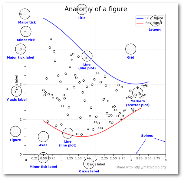
Elements in a figure in object-oriented interface
The following figure taken from https://pbpython.com/effective-matplotlib.html explains the components of a figure pretty well:
Let’s look at one simple example of how to create a line chart with object-oriented interface.
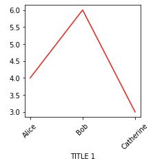
fig, ax = plt.subplots(figsize=(3,3))
ax.plot(['Alice','Bob','Catherine'], [4,6,3], color='r')
ax.set_xlabel('TITLE 1')
for tick in ax.get_xticklabels():
    tick.set_rotation(45)
plt.show()
In the codes above, we created an axes object, created a line plot on top of it, added a title, and rotated all the x-tick labels by 45 degrees counterclockwise.
Check out the official API to see how to manipulate axes objects: https://matplotlib.org/api/axes_api.html
A few common types of plots
After getting a rough idea about how Matplotlib works, it’s time to check out some commonly seen plots. They are
Scatter plots (x: Numerical #1, y: Numerical #2),
Line plots (x: Categorical - ordinal#1, y: Numerical #1) [Thanks to Michael Arons for pointing out an issue in the previous figure],
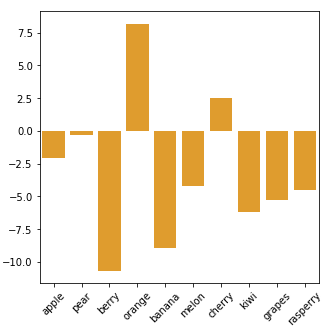
Bar plots (x: Categorical #1, y: Numerical #1). Numerical #1 is often the count of Categorical #1.
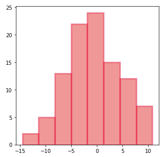
Histogram (x: Numerical #1, y: Numerical #2). Numerical #1 is combined into groups (converted to a categorical variable), and Numerical #2 is usually the count of this categorical variable.
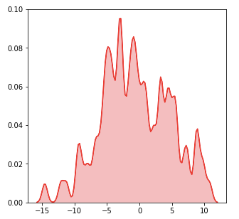
Kernel density plot (x: Numerical #1, y: Numerical #2). Numerical #2 is the frequency of Numerical #1.
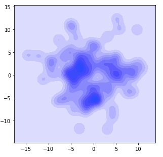
2-D kernel density plot (x: Numerical #1, y: Numerical #2, color: Numerical #3). Numerical #3 is the joint frequency of Numerical #1 and Numerical #2.
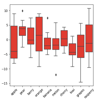
Box plot (x: Categorical #1, y: Numerical #1, marks: Numerical #2). Box plot shows the statistics of each value in Categorical #1 so we’ll get an idea of the distribution in the other variable. y-value: the value for the other variable; marks: showing how these values are distributed (range, Q1, median, Q3).
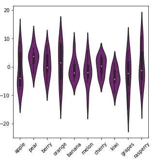
Violin plot (x: Categorical #1, y: Numerical #1, Width/Mark: Numerical #2). Violin plot is sort of similar to box plot but it shows the distribution better.
Heat map (x: Categorical #1, y: Categorical #2, Color: Numerical #1). Numerical #1 could be the count for Categorical #1 and Categorical #2 jointly, or it could be other numerical attributes for each value in the pair (Categorical #1, Categorical #2).

To learn how to plot these figures, the readers can check out the seaborn APIs by googling for the following list:
sns.barplot / sns.distplot / sns.lineplot / sns.kdeplot / sns.violinplot
sns.scatterplot / sns.boxplot / sns.heatmap
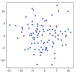
I’ll give two example codes showing how 2D kde plots / heat map are generated in object-oriented interface.
# 2D kde plots
import numpy as np
import matplotlib.pyplot as plt
import seaborn as sns
np.random.seed(1)
numerical_1 = np.random.randn(100)
np.random.seed(2)
numerical_2 = np.random.randn(100)
fig, ax = plt.subplots(figsize=(3,3))
sns.kdeplot(data=numerical_1,
            data2= numerical_2,
            ax=ax,
            shade=True,
            color="blue",
            bw=1)
plt.show()
The key is the argument ax=ax. When running .kdeplot() method, seaborn would apply the changes to ax, an ‘axes’ object.
# heat map
import numpy as np
import pandas as pd
import matplotlib.pyplot as plt
import seaborn as sns
df = pd.DataFrame(dict(categorical_1=['apple', 'banana', 'grapes',
                                      'apple', 'banana', 'grapes',
                                      'apple', 'banana', 'grapes'],
                  categorical_2=['A','A','A','B','B','B','C','C','C'],
                  value=[10,2,5,7,3,15,1,6,8]))
pivot_table = df.pivot("categorical_1", "categorical_2", "value")
# try printing out pivot_table to see what it looks like!
fig, ax = plt.subplots(figsize=(5,5))
sns.heatmap(data=pivot_table,
            cmap=sns.color_palette("Blues"),
            ax=ax)

plt.show()
Increase the dimension of your plots
For these basic plots, only limited amount of information can be displayed (2–3 variables). What if we’d like to show more info to these plots? Here are a few ways.
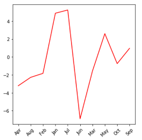
- Overlay plots
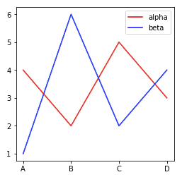
If several line charts share the same x and y variables, you can call Seaborn plots multiple times and plot all of them on the same figure. In the example below, we added one more categorical variable [value = alpha, beta] in the plot with overlaying plots.
fig, ax = plt.subplots(figsize=(4,4))
sns.lineplot(x=['A','B','C','D'],
y=[4,2,5,3],
color='r',
ax=ax)
sns.lineplot(x=['A','B','C','D'],
y=[1,6,2,4],
color='b',
ax=ax)
ax.legend(['alpha', 'beta'], facecolor='w')
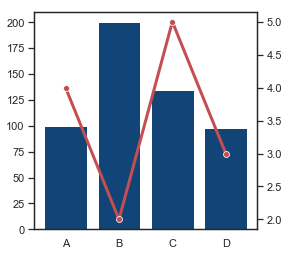
plt.show()Or, we can combine a bar chart and a line chart with the same x-axis but different y-axis:
sns.set(style="white", rc={"lines.linewidth": 3})
fig, ax1 = plt.subplots(figsize=(4,4))
ax2 = ax1.twinx()
sns.barplot(x=['A','B','C','D'],
            y=[100,200,135,98],
            color='#004488',
            ax=ax1)
sns.lineplot(x=['A','B','C','D'],
             y=[4,2,5,3],
             color='r',
             marker="o",
             ax=ax2)
plt.show()
sns.set()
A few comments here. Because the two plots have different y-axis, we need to create another ‘axes’ object with the same x-axis (using .twinx()) and then plot on different ‘axes’. sns.set(…) is to set specific aesthetics for the current plot, and we run sns.set() in the end to set everything back to default settings.
Combining different barplots into one grouped barplot also adds one categorical dimension to the plot (one more categorical variable).
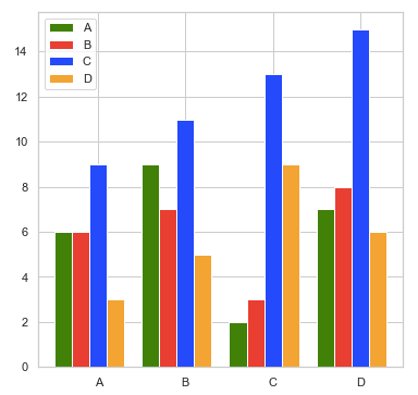
import matplotlib.pyplot as plt
categorical_1 = ['A', 'B', 'C', 'D']
colors        = ['green', 'red', 'blue', 'orange']
numerical = [[6, 9, 2, 7],
             [6, 7, 3, 8],
             [9, 11, 13, 15],
             [3, 5, 9, 6]]
number_groups = len(categorical_1)
bin_width = 1.0/(number_groups+1)
fig, ax = plt.subplots(figsize=(6,6))
for i in range(number_groups):
    ax.bar(x=np.arange(len(categorical_1)) + i*bin_width,
           height=numerical[i],
           width=bin_width,
           color=colors[i],
           align='center')
ax.set_xticks(np.arange(len(categorical_1)) + number_groups/(2*(number_groups+1)))
# number_groups/(2*(number_groups+1)): offset of xticklabel
ax.set_xticklabels(categorical_1)
ax.legend(categorical_1, facecolor='w')
plt.show()
In the code example above, you can customize variable names, colors, and figure size. number_groups and bin_width are calculated based on the input data. I then wrote a for-loop to plot the bars, one color at a time, and set the ticks and legends in the very end.
2. Facet — mapping dataset into multiple axes, and they differ by one or two categorical variable(s). The reader could find a bunch examples in https://seaborn.pydata.org/generated/seaborn.FacetGrid.html
3. Color / Shape / Size of nodes in a scatter plot: The following code example taken from Seaborn Scatter Plot API shows how it works. (https://seaborn.pydata.org/generated/seaborn.scatterplot.html)
import seaborn as sns
tips = sns.load_dataset("tips")
ax = sns.scatterplot(x="total_bill", y="tip",
                     hue="size", size="size",
                     sizes=(20, 200), hue_norm=(0, 7),
                     legend="full", data=tips)
plt.show()
Partition the figure using GridSpec
One of the advantages for object-oriented interface is that we can easily partition our figure into several subplots and manipulate each subplot with ‘axes’ API.
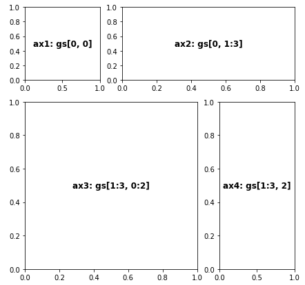
fig = plt.figure(figsize=(7,7))
gs = gridspec.GridSpec(nrows=3,
                       ncols=3,
                       figure=fig,
                       width_ratios= [1, 1, 1],
                       height_ratios=[1, 1, 1],
                       wspace=0.3,
                       hspace=0.3)
ax1 = fig.add_subplot(gs[0, 0])
ax1.text(0.5, 0.5, 'ax1: gs[0, 0]', fontsize=12, fontweight="bold", va="center", ha="center")  # adding text to ax1
ax2 = fig.add_subplot(gs[0, 1:3])
ax2.text(0.5, 0.5, 'ax2: gs[0, 1:3]', fontsize=12, fontweight="bold", va="center", ha="center")
ax3 = fig.add_subplot(gs[1:3, 0:2])
ax3.text(0.5, 0.5, 'ax3: gs[1:3, 0:2]', fontsize=12, fontweight="bold", va="center", ha="center")
ax4 = fig.add_subplot(gs[1:3, 2])
ax4.text(0.5, 0.5, 'ax4: gs[1:3, 2]', fontsize=12, fontweight="bold", va="center", ha="center")
plt.show()
In the example, we first partition the figure into 3*3 = 9 small boxes with gridspec.GridSpec(), and then define a few axes objects. Each axes object could contain one or more boxes. Say in the codes above, gs[0, 1:3] = gs[0, 1] + gs[0, 2] is assigned to axes object ax2. wspace and hspace are parameters controlling the space between plots.
Create advanced visualizations
With some tutorials from the previous sections, it’s time to produce some cool stuffs. Let’s download the Analytics Vidhya Black Friday Sales data from
https://www.kaggle.com/mehdidag/black-friday and do some easy data preprocessing:
df = pd.read_csv('BlackFriday.csv', usecols = ['User_ID', 'Gender', 'Age', 'Purchase'])
df_gp_1 = df[['User_ID', 'Purchase']].groupby('User_ID').agg(np.mean).reset_index()
df_gp_2 = df[['User_ID', 'Gender', 'Age']].groupby('User_ID').agg(max).reset_index()
df_gp = pd.merge(df_gp_1, df_gp_2, on = ['User_ID'])
You’ll then get a table of user ID, gender, age, and the average price of items in each customer’s purchase.
Step 1. Goal
We’re curious about how age and gender would affect the average purchased item price during Black Friday, and we hope to see the price distribution as well. We also want to know the percentages for each age group.
Step 2. Variables
We’d like to include age group (categorical), gender (categorical), average item price (numerical), and the distribution of average item price (numerical) in the plot. We need to include another plot with the percentage for each age group (age group + count/frequency).
To show average item price + its distributions, we can go with kernel density plot, box plot, or violin plot. Among these, kde shows the distribution the best. We then plot two or more kde plots in the same figure and then do facet plots, so age group and gender info can be both included. For the other plot, a bar plot can do the job well.
Step 3. Visualization
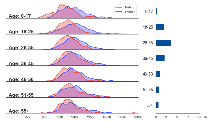
Once we have a plan about the variables, we could then think about how to visualize it. We need to do figure partitions first, hide some boundaries, xticks, and yticks, and then add a bar chart to the right.
The plot below is what we’re going to create. From the figure, we can clearly see that men tend to purchase more expensive items then women do based on the data, and elder people tend to purchase more expensive items (the trend is clearer for the top 4 age groups). We also found that people with age 18–45 are the major buyers in Black Friday sales.
The codes below generate the plot (explanations are included in the comments):
freq = ((df_gp.Age.value_counts(normalize = True).reset_index().sort_values(by = 'index').Age)*100).tolist()
number_gp = 7
# freq = the percentage for each age group, and there’re 7 age groups.
def ax_settings(ax, var_name, x_min, x_max):
    ax.set_xlim(x_min,x_max)
    ax.set_yticks([])

    ax.spines['left'].set_visible(False)
    ax.spines['right'].set_visible(False)
    ax.spines['top'].set_visible(False)

    ax.spines['bottom'].set_edgecolor('#444444')
    ax.spines['bottom'].set_linewidth(2)

    ax.text(0.02, 0.05, var_name, fontsize=17, fontweight="bold", transform = ax.transAxes)
    return None
# Manipulate each axes object in the left. Try to tune some parameters and you'll know how each command works.
fig = plt.figure(figsize=(12,7))
gs = gridspec.GridSpec(nrows=number_gp,
                       ncols=2,
                       figure=fig,
                       width_ratios= [3, 1],
                       height_ratios= [1]*number_gp,
                       wspace=0.2, hspace=0.05
                      )
ax = [None]*(number_gp + 1)
features = ['0-17', '18-25', '26-35', '36-45', '46-50', '51-55', '55+']
# Create a figure, partition the figure into 7*2 boxes, set up an ax array to store axes objects, and create a list of age group names.
for i in range(number_gp):
    ax[i] = fig.add_subplot(gs[i, 0])

    ax_settings(ax[i], 'Age: ' + str(features[i]), -1000, 20000)

    sns.kdeplot(data=df_gp[(df_gp.Gender == 'M') & (df_gp.Age == features[i])].Purchase,
            ax=ax[i], shade=True, color="blue",  bw=300, legend=False)
    sns.kdeplot(data=df_gp[(df_gp.Gender == 'F') & (df_gp.Age == features[i])].Purchase,
            ax=ax[i], shade=True, color="red",  bw=300, legend=False)

    if i < (number_gp - 1):
        ax[i].set_xticks([])
# this 'for loop' is to create a bunch of axes objects, and link them to GridSpec boxes. Then, we manipulate them with sns.kdeplot() and ax_settings() we just defined.
ax[0].legend(['Male', 'Female'], facecolor='w')
# adding legends on the top axes object
ax[number_gp] = fig.add_subplot(gs[:, 1])
ax[number_gp].spines['right'].set_visible(False)
ax[number_gp].spines['top'].set_visible(False)
ax[number_gp].barh(features, freq, color='#004c99', height=0.4)
ax[number_gp].set_xlim(0,100)
ax[number_gp].invert_yaxis()
ax[number_gp].text(1.09, -0.04, '(%)', fontsize=10, transform = ax[number_gp].transAxes)
ax[number_gp].tick_params(axis='y', labelsize = 14)
# manipulate the bar plot on the right. Try to comment out some of the commands to see what they actually do to the bar plot.


plt.show()
Plots like this one are also called ‘Joy plot’ or ‘Ridgeline plot’. If you try to use some joyplot packages to plot the same figure, you’ll find it a bit difficult to do because two density plots are included in the each subplot.
Hope this is a joyful reading for you.