Time series data consists of data points attached to sequential time stamps. Daily sales, hourly temperature values, and second-level measurements in a chemical process are some examples of time series data.
Time series data has different characteristics than ordinary tabular data. Thus, time series analysis has its own dynamics and can be considered as a separate field. There are books over 500 pages to cover time series analysis concepts and techniques in depth.
Pandas was created by Wes Mckinney to provide an efficient and flexible tool to work with financial data which is kind of a time series. In this article, we will go over 4 Pandas functions that can be used for time series analysis.
We need data for the examples. Let’s start with creating our own time series data.
import numpy as np
import pandas as pd
df = pd.DataFrame({
   "date": pd.date_range(start="2020-05-01", periods=100, freq="D"),
   "temperature": np.random.randint(18, 30, size=100) +
                  np.random.random(100).round(1)
})
df.head()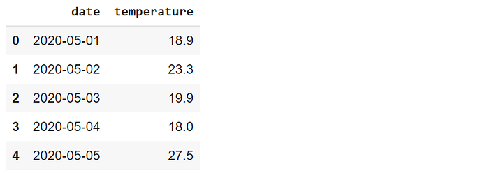
(image by author)
We have created a data frame that contains temperature measurements during a period of 100 days. The date_range function of Pandas can be used for generating a date range with customized frequency. The temperature values are generated randomly using Numpy functions.
We can now start on the functions.
1. Shift
It is a common operation to shift time series data. We may need to make a comparison between lagged or lead features. In our data frame, we can create a new feature that contains the temperature of the previous day.
df["temperature_lag_1"] = df["temperature"].shift(1)
df.head()
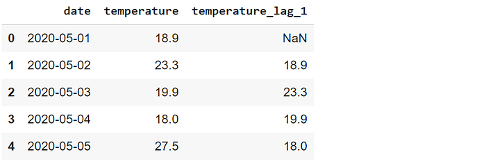
(image by author)
The scalar value passed to the shift function indicates the number of periods to shift. The first row of the new column is filled with NaN because there is no previous value for the first row.
The fill_value parameter can be used for filling the missing values with a scalar. Let’s replace the NaN with the average value of the temperature column.
df["temperature_lag_1"] = df["temperature"]\
.shift(1, fill_value = df.temperature.mean())
df.head()
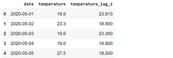
(image by author)
If you are interested in the future values, you can shift backwards by passing negative values to the shift function. For instance, “-1” brings the temperature in the next day.
2. Resample
Another common operation performed on time series data is resampling. It involves in changing the frequency of the periods. For instance, we may be interested in the weekly temperature data rather than daily measurements.
The resample function creates groups (or bins) of a specified internal. Then, we can apply aggregation functions to the groups to calculate the value based on resampled frequency.
Let’s calculate the average weekly temperatures. The first step is to resample the data to week level. Then, we will apply the mean function to calculate the average.
df_weekly = df.resample("W", on="date").mean()
df_weekly.head()
(image by author)
The first parameter specifies the frequency for resampling. “W” stands for week, surprisingly. If the data frame does not have a datetime index, the column that contains the date or time related information needs to be passed to the on parameter.
3. Asfreq
The asfreq function provides a different technique for resampling. It returns the value at the end of the specified interval. For instance, asfreq(“W”)returns the value on the last day of each week.
In order to use the asfreq function, we should set the date column as the index of the data frame.
df.set_index("date").asfreq("W").head()(image by author)
Since we are getting a value at a specific day, it is not necessary to apply an aggregation function.
4. Rolling
The rolling function can be used for calculating moving average which is a highly common operation for time series data. It creates a window of a particular size. Then, we can use this window to make calculations as it rolls through the data points.
The figure below explains the concept of rolling.
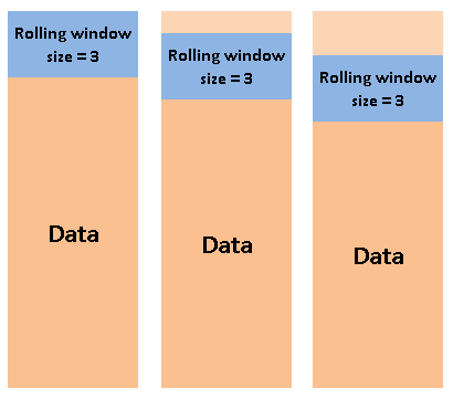
(image by author)
Let’s create a rolling window of 3 and use it to calculate the moving average.
df.set_index("date").rolling(3).mean().head()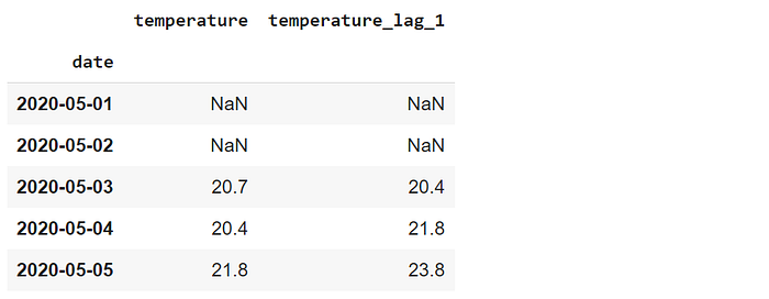
(image by author)
For any day, the values show the average of the day and the previous 2 days. The values of the first 3 days are 18.9, 23.8, and 19.9. Thus, the moving average on the third day is the average of these values which is 20.7.
The first 2 values are NaN because they do not have previous 2 values. We can also use this rolling window to cover the previous and next day for any given day. It can be done by setting the center parameter as true.
df.set_index("date").rolling(3, center=True).mean().head()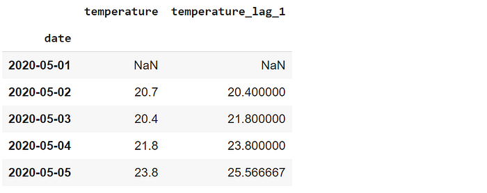
(image by author)
The values of the first 3 days are 18.9, 23.8, and 19.9. Thus, the moving average in the second day is the average of these 3 values. In this setting, only the first value is NaN because we only need 1 previous value.
Conclusion
We have covered 4 Pandas functions that are commonly used in time series analysis. Predictive analytics is an essential part of data science. Time series analysis is at the core of many problems that predictive analytics aims to solve. Hence, if you plan to work on predictive analytics, you should definitely learn how to handle time series data.
Thank you for reading. Please let me know if you have any feedback.