
F.G.O. Stuart (1843–1923) / Public domain
RMS Titanic was a British passenger liner operated by the White Star Line that sank in the North Atlantic Ocean in the early morning hours of April 15, 1912, after striking an iceberg during her maiden voyage from Southampton to New York City. Of the estimated 2,224 passengers and crew aboard, more than 1,500 died, making the sinking one of modern history’s deadliest peacetime commercial marine disasters.
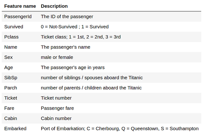
What we want now is to create a machine learning model that is able to predict who would survive Titanic’s shipwreck. For that we will use this dataset from Kaggle — there is also a Kaggle competition for this task which is a good place to get started with Kaggle competitions. This dataset contains the following information about the passengers:
Exploratory Analysis
Now, before doing any machine learning on this dataset, it is a good practice to do some exploratory analysis and see how our data looks like. We also want to prepare/clean it along the way.
import numpy as np
import pandas as pd
df = pd.read_csv('train.csv')
df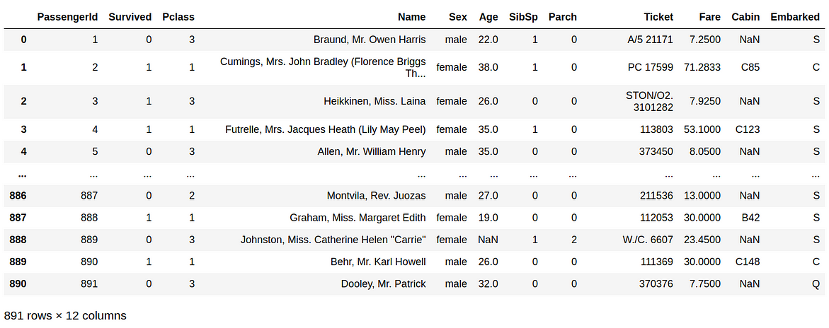
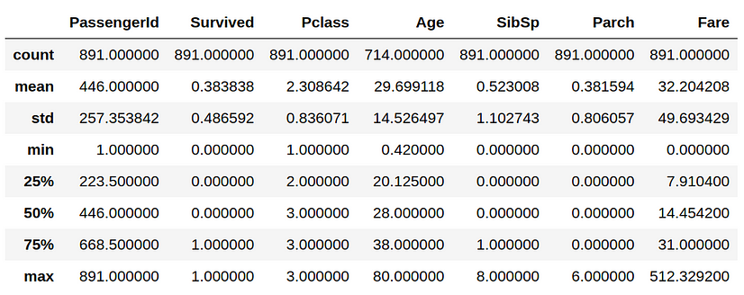
df.describe()
What do we see in our data at first glance? We see that the PassengerId column has an unique number associated with each passenger. This field can easily be used by machine learning algorithms to just memorize the outcomes for each passenger without the ability to generalize. Also, there is the Name variable which I personally don’t think it determines in any way if one person survived or not. So, we will delete these two variables.
del df['PassengerId']
del df['Name']
Now, let’s see if we have missing values and how many they are.
df.isnull().sum()
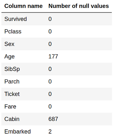
Out of 891 samples, 687 have null values for the Cabin variable. There are too many missing values for this variable to be able to make use of it. We will delete it.
del df['Cabin']
We don’t want to delete the other two columns as they have few missing values, we will augment them.
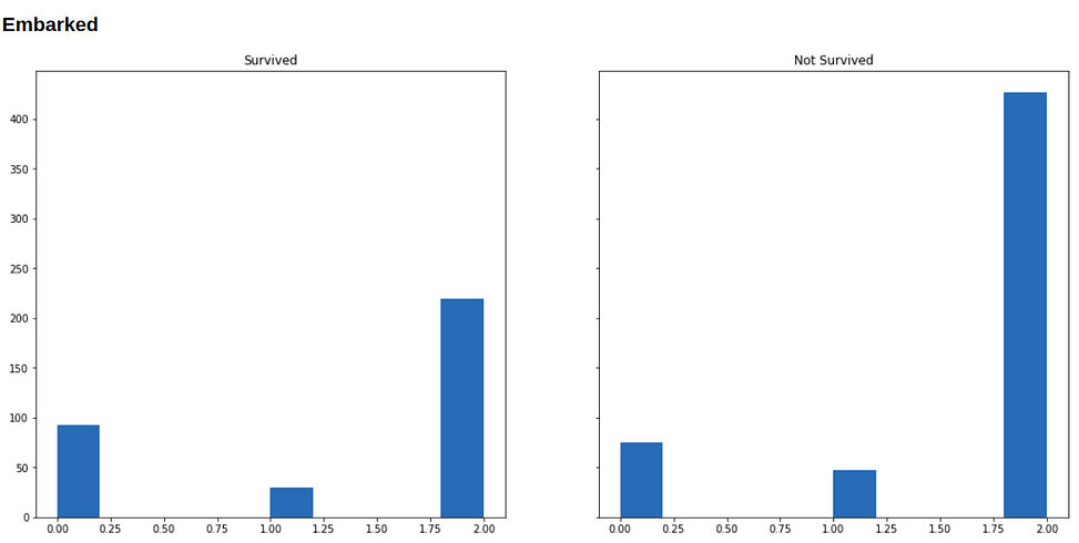
For the Embarked variable, as it is a categorical variable, we will look at the counts of each category and replace the 2 null values with the category that has most items.
df['Embarked'].value_counts()
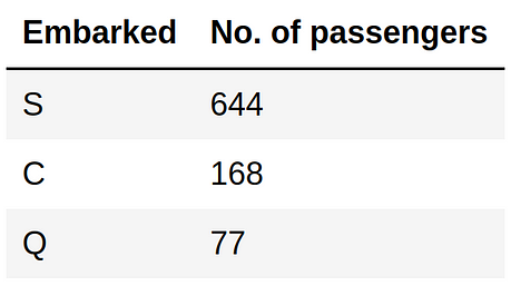
The most frequent value for Embarked is ‘S’, so we will use it to replace the null values.
df['Embarked'].loc[pd.isnull(df['Embarked'])] = 'S'
For age we will replace missing values with the average age.
mean_age_train = np.mean(df['Age'].loc[pd.isnull(df['Age']) == False].values)
df['Age'].loc[pd.isnull(df['Age'])] = mean_age_train
Note that we should store everything that we learn from our training data, such as Embarked class frequency or Age mean, as we will use this information when making predictions in case there are also missing values in test data.
We will also compute and store Fare mean in case we need it on test data.
mean_fare_train = np.mean(df['Fare'].loc[pd.isnull(df['Fare']) == False].values)
We got rid of null values, now let’s see what’s next.
Ordinal Encoding
Machine learning algorithms don’t work with text (at least not directly), we need to convert all strings with numbers. We will use ordinal encoding for this conversion. Ordinal encoding is a way to convert a categorical variable into numbers by assigning each category a number. We’re going to use Scikit-Learn’s OrdinalEncoder to apply this transformation on variables Sex, Ticket, Embarked.
Before that, we will backup our current data format for future use.
df_bkp = df.copy()
from sklearn.preprocessing import OrdinalEncoder
df['Sex'] = OrdinalEncoder().fit_transform(df['Sex'].values.reshape((-1, 1)))
df['Ticket'] = OrdinalEncoder().fit_transform(df['Ticket'].values.reshape((-1, 1)))
df['Embarked'] = OrdinalEncoder().fit_transform(df['Embarked'].values.reshape((-1, 1)))
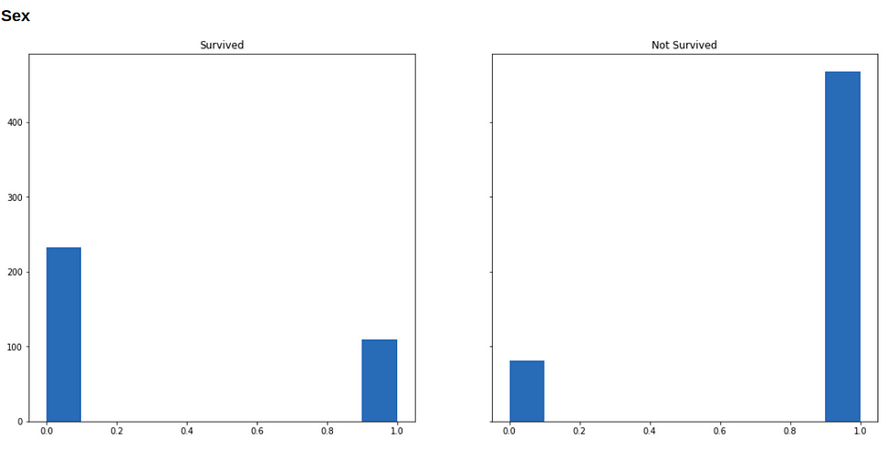
Visualizations
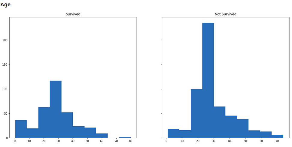
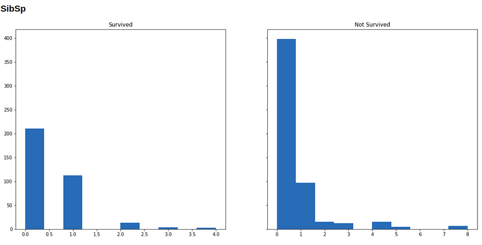
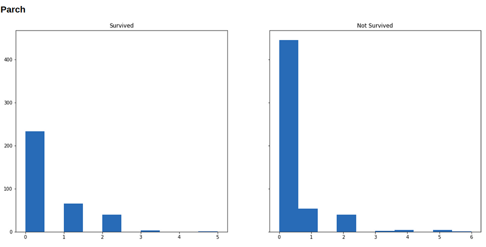
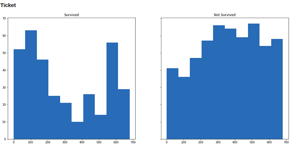
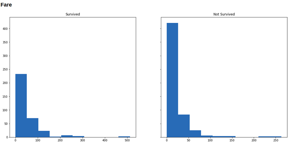
Now we will visualize our data to see how the distribution of our variables varies across survived and not-survived classes.
Below are histograms for each variable in our dataset (along with the code that generated it), in the left is the subset of people who survived, and in the right who didn’t survive.
import matplotlib.pyplot as plt
from IPython.display import display, Markdown
def show(txt):
    # this function is for printing markdown in jupyter notebook
    display(Markdown(txt))
for i in range(1, 9):
    show(f'### {df.columns[i]}')
    f, (survived, not_survived) = plt.subplots(1, 2, sharey=True, figsize=(18, 8))
    survived.hist(df.iloc[np.where(df['Survived'] == 1)[0], i])
    survived.set_title('Survived')
not_survived.hist(df.iloc[np.where(df['Survived'] == 0)[0], i])
    not_survived.set_title('Not Survived')
    plt.show()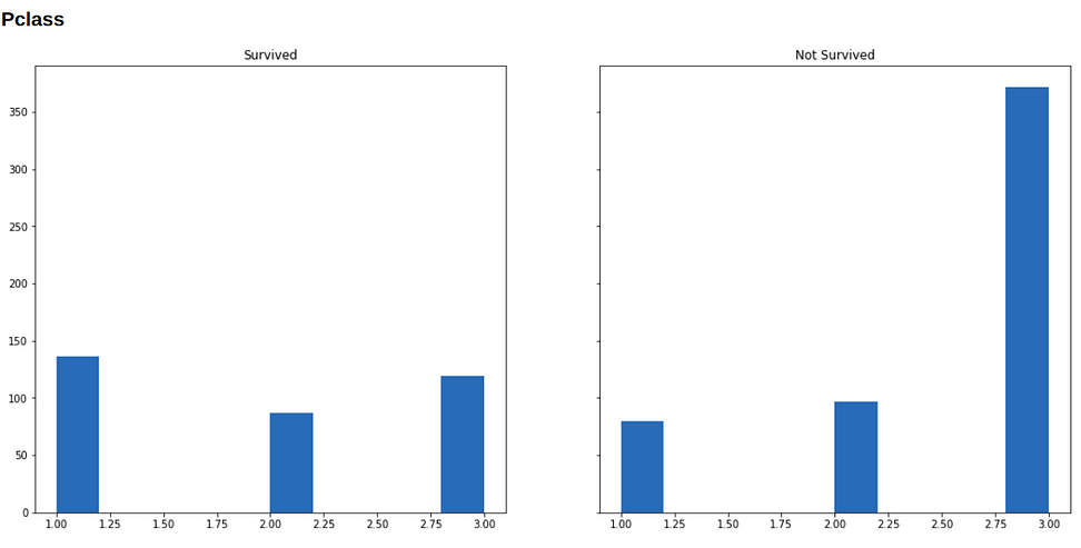
Running Machine Learning on this data format
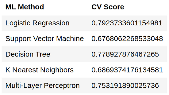
Now, we will try a couple of machine learning methods on our dataset to see what results we get. The machine learning methods that we will use are:
- Logistic Regression
- Support Vector Machine
- Decision Tree
- K Nearest Neighbors
- Multi-Layer Perceptron
Instead of choosing a fixed validation set to estimate the accuracy of the test set, we will use (5-fold) cross validation with Scikit-Learn’s cross_val_score which returns an array with scores for each cross validation iteration.
from sklearn.model_selection import cross_val_score
from sklearn.linear_model import LogisticRegression
from sklearn.svm import SVC
from sklearn.tree import DecisionTreeClassifier
from sklearn.neighbors import KNeighborsClassifier
from sklearn.neural_network import MLPClassifier
X = df.iloc[:, 1:].values
y = df.iloc[:, 0].values
# Logistic Regression
lr = LogisticRegression()
lr_score = np.mean(cross_val_score(lr, X, y))
print(f'Logistic Regression: {lr_score}')
# Support Vector Machine
svc = SVC()
svc_score = np.mean(cross_val_score(svc, X, y))
print(f'Support Vector Machine: {svc_score}')
# Decision Tree
dtc = DecisionTreeClassifier()
dtc_score = np.mean(cross_val_score(dtc, X, y))
print(f'Decision Tree: {dtc_score}')
# K Nearest Neighbors
knc = KNeighborsClassifier()
knc_score = np.mean(cross_val_score(knc, X, y))
print(f'K Nearest Neighbors: {knc_score}')
# Multi-Layer Perceptron
mlpc = MLPClassifier()
mlpc_score = np.mean(cross_val_score(mlpc, X, y))
print(f'Multi-Layer Perceptron: {mlpc_score}')
Running this code we got the following results:
Feature Engineering
Let’s see if we can improve the accuracy by working on our dataset’s features. For that, we will restore first to the backup we made before applying ordinal encoding.
df = df_bkp.copy()
One-Hot Encoding
Instead of ordinal encoding, now we want to apply one-hot encoding to our categorical variables. With one-hot encoding, instead of assigning each class a number, we assign a vector with all 0’s except for one position specific to that class in which we put a 1. That is, we transform each class into a variable on its own that takes the value 0 or 1. We will apply one-hot encoding on the variables Pclass, Sex, Ticket and Embarked using Scikit-Learn’s OneHotEncoder.
from sklearn.preprocessing import OneHotEncoder
# Pclass
pclass_transf = OneHotEncoder(sparse=False, dtype=np.uint8, handle_unknown='ignore')
pclass_transf.fit(df['Pclass'].values.reshape((-1, 1)))
pclass = pclass_transf.transform(df['Pclass'].values.reshape((-1, 1)))
df['Pclass0'] = pclass[:, 0]
df['Pclass1'] = pclass[:, 1]
df['Pclass2'] = pclass[:, 2]
del df['Pclass']
# Sex
gender_transf = OneHotEncoder(sparse=False, dtype=np.uint8, handle_unknown='ignore')
gender_transf.fit(df['Sex'].values.reshape((-1, 1)))
gender = gender_transf.transform(df['Sex'].values.reshape((-1, 1)))
df['Male'] = gender[:, 0]
df['Female'] = gender[:, 1]
del df['Sex']
# Ticket
ticket_transf = OneHotEncoder(sparse=False, dtype=np.uint8, handle_unknown='ignore')
ticket_transf.fit(df['Ticket'].values.reshape((-1, 1)))
ticket = ticket_transf.transform(df['Ticket'].values.reshape((-1, 1)))
for i in range(ticket.shape[1]):
    df[f'Ticket{i}'] = ticket[:, i]
del df['Ticket']
# Embarked
embarked_transf = OneHotEncoder(sparse=False, dtype=np.uint8, handle_unknown='ignore')
embarked_transf.fit(df['Embarked'].values.reshape((-1, 1)))
embarked = embarked_transf.transform(df['Embarked'].values.reshape((-1, 1)))
for i in range(embarked.shape[1]):
    df[f'Embarked{i}'] = embarked[:, i]
del df['Embarked']
Scaling to [0, 1] range
We also want to scale the numerical variables to [0, 1] range. For that we will use MinMaxScaler which scales the variables so that the minimum value is moved to 0, the maximum to 1 and other intermediary values are scaled accordingly in between 0, 1. We will apply this transformation to variables Age, SibSp, Parch, Fare.
from sklearn.preprocessing import MinMaxScaler
age_transf = MinMaxScaler().fit(df['Age'].values.reshape(-1, 1))
df['Age'] = age_transf.transform(df['Age'].values.reshape(-1, 1))
sibsp_transf = MinMaxScaler().fit(df['SibSp'].values.reshape(-1, 1))
df['SibSp'] = sibsp_transf.transform(df['SibSp'].values.reshape(-1, 1))
parch_transf = MinMaxScaler().fit(df['Parch'].values.reshape(-1, 1))
df['Parch'] = parch_transf.transform(df['Parch'].values.reshape(-1, 1))
fare_transf = MinMaxScaler().fit(df['Fare'].values.reshape(-1, 1))
df['Fare'] = fare_transf.transform(df['Fare'].values.reshape(-1, 1))
Doing Machine Learning on this new data format
Now we will run the same machine learning algorithms on this new data format to see what results we get.
X = df.iloc[:, 1:].values
y = df.iloc[:, 0].values
# Logistic Regression
lr = LogisticRegression()
lr_score = np.mean(cross_val_score(lr, X, y))
print(f'Logistic Regression: {lr_score}')
# Support Vector Machine
svc = SVC()
svc_score = np.mean(cross_val_score(svc, X, y))
print(f'Support Vector Machine: {svc_score}')
# Decision Tree
dtc = DecisionTreeClassifier()
dtc_score = np.mean(cross_val_score(dtc, X, y))
print(f'Decision Tree: {dtc_score}')
# K Nearest Neighbors
knc = KNeighborsClassifier()
knc_score = np.mean(cross_val_score(knc, X, y))
print(f'K Nearest Neighbors: {knc_score}')
# Multi-Layer Perceptron
mlpc = MLPClassifier()
mlpc_score = np.mean(cross_val_score(mlpc, X, y))
print(f'Multi-Layer Perceptron: {mlpc_score}')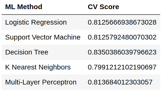
After we engineered our features in this way we got an significant improvement in the accuracy of all classifiers. The best classifier among them being Decision Tree Classifier. Now we try to improve it by doing hyper-parameter tuning using GridSearchCV.
Hyper-Parameter Tuning
from sklearn.model_selection import GridSearchCV
dtc = DecisionTreeClassifier()
params = {
    'max_depth': list(range(2, 151)),
    'min_samples_split': list(range(2, 15))
}
clf = GridSearchCV(dtc, params)
clf.fit(X, y)
print(f'Best params: {clf.best_params_}')
print(f'Best score: {clf.best_score_}')
The parameters that we got are:
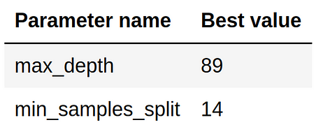
And the score that we got is 84.40%, an improvement of 0.9% after hyperparameter tuning.